What Is Interest During Construction?
Interest During Construction is the interest that is applied in the construction period. It is calculated on the debt for the project. You will need to know the debt, the interest rate and some other variables to calculate Interest During Construction.
Step by Step Calculation of Interest During Construction in Excel
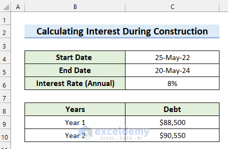
We will use the following sample dataset for illustration. The Start Date and the End Date of the construction period are given. The annual Interest Rate is 8%. And the Debt in Year 1 is $88,500 and in Year 2 is $90,550.
Step 1 – Select Drawdown Mode and Frequency
- Create a section for entering the Drawdown Mode and Drawdown Frequency.
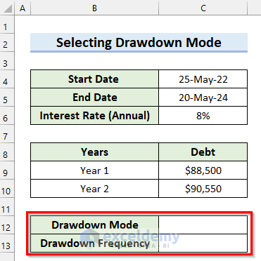
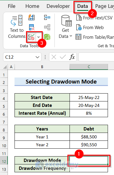
- Select the cell where you want to show the Drawdown Mode. We have selected cell C12.
- Go to the Data tab.
- Select Data Validation.
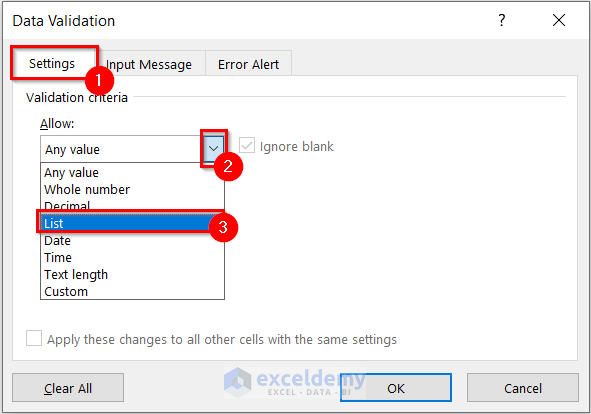
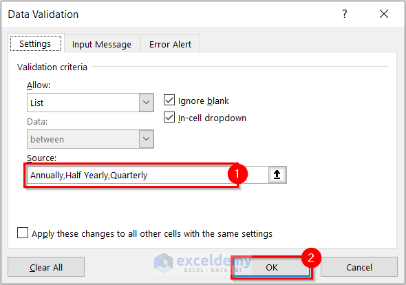
- The Data Validation dialog box will appear.
- Select the Settings tab.
- Click on the drop-down button for Allow from Validation criteria.
- Select List.
- Enter the options you want in the Source section.
- Select OK.
- You will see a drop-down button has been inserted in your selected cell which is cell C12.
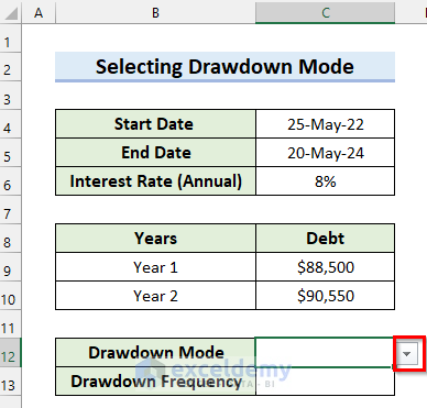
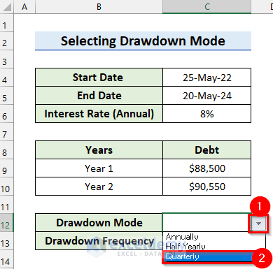
- To select Drawdown Mode, first Click on the drop-down button.
- Select the mode you want. we have selected Quarterly.
- You will see that Quarterly is showing as Drawdown Mode.
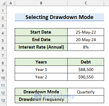
- Select the cell where you want to show the Drawdown Frequency. we have selected cell C13.
- In cell C13, enter the following formula.
=IF(C12="Annually",12,IF(C12="Half Yearly",6,3))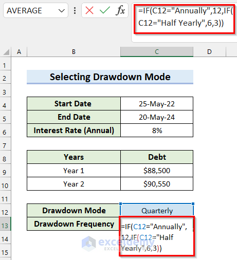
- Press Enter and you will get your Drawdown Frequency.
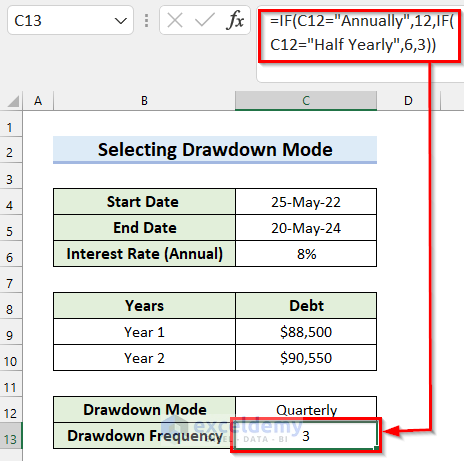
How Does the Formula Work?
- IF(C12=”Half Yearly”,6,3):the IF function returns 6 if the logical_test is True. Otherwise, it returns 3.
- IF(C12=”Annually”,12,IF(C12=”Half Yearly”,6,3)): the IF function returns 12 if the logical_test is True. Otherwise, it will go to the next IF function.
Step 2 – Create Table for Interest During Construction
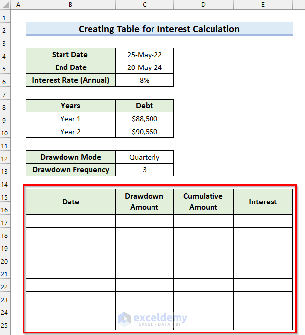
- Create a table with 4 columns.
- Name the columns as Date, Drawdown Amount, Cumulative Amount and Interest.
Step 3 – Insert Dates into Table
We will insert the Dates for every drawdown period for the project.
- Select the cell where you want the first Date.
- Enter the following formula in that selected cell.
=C4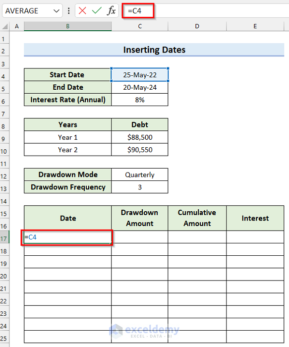
- Press Enter to get the Date.
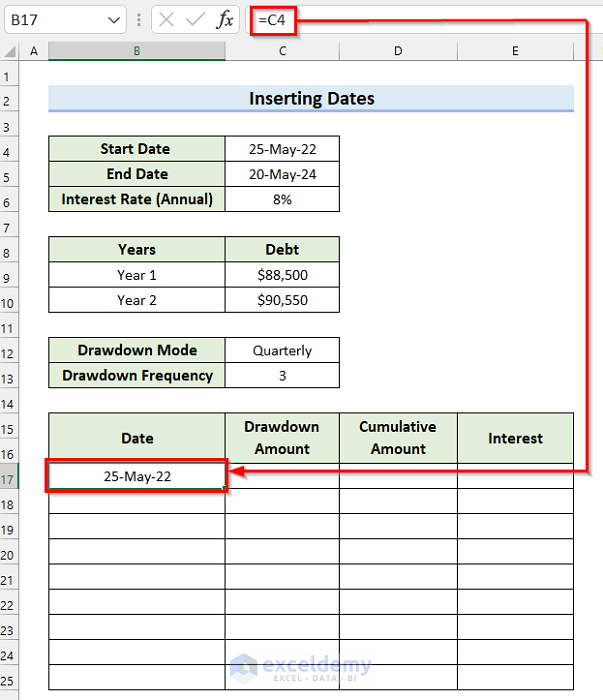
- Select the cell where you want the second Date. we have selected cell B18.
- In cell B18 enter the following formula.
=IF(B17<$C$5,EDATE(B17,$C$13),"")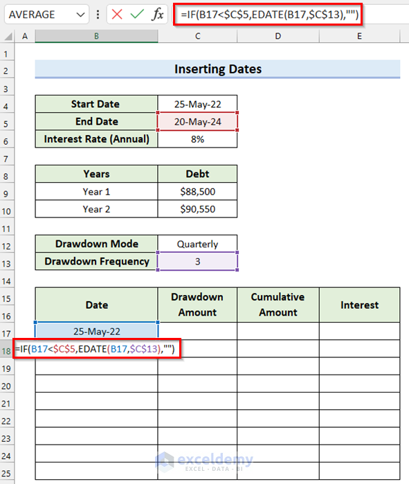
- Press Enter to get the Date.
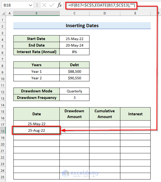
- Drag the Fill Handle down to copy the formula to the other cells.
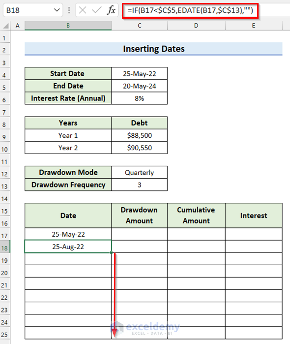
How Does the Formula Work?
- EDATE(B17,$C$13): In the EDATE function, we selected B17 as start_date and C13 as months. The formula will return the date after the months in cell C13 from the date in cell B17.
- IF(B17<$C$5,EDATE(B17,$C$13),””): The IF function will check if the value in cell C5 is less than the value in cell C5. If the logical_test is True then the formula returns the Date generated by the EDATE Otherwise, it returns blank.
- You can see that we have copied the formula to the other cells and got the desired output.
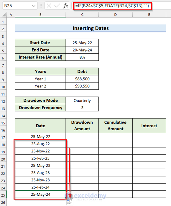
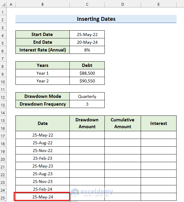
- In the following image, you can see that the last date is after the End Date. So, we will delete this date.
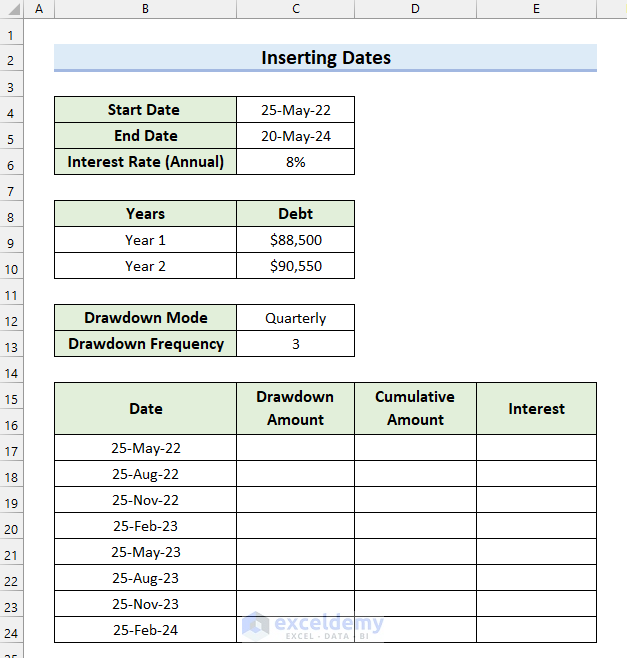
- This is how the table looks like at this stage.
Read More: How to Calculate Interest Between Two Dates in Excel
Step 4 – Calculate Drawdown Amount
- Select the cell where you want to calculate the Drawdown Amount for Year 1.
- Enter the following code in that selected cell.
=$C$9/(12/$C$13)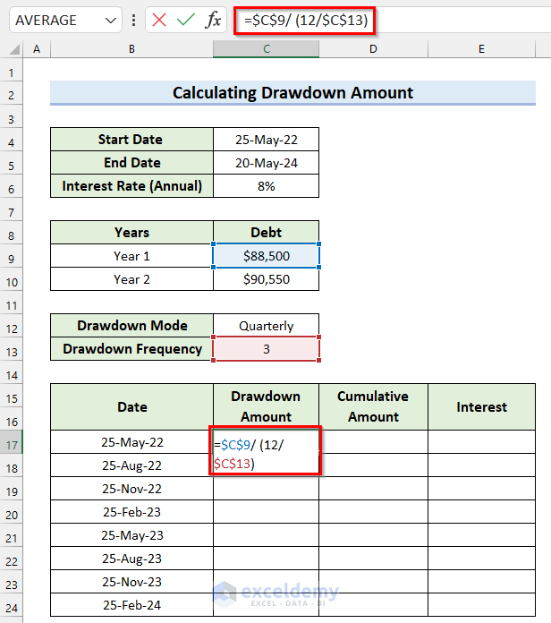
- Press Enter to get the result.
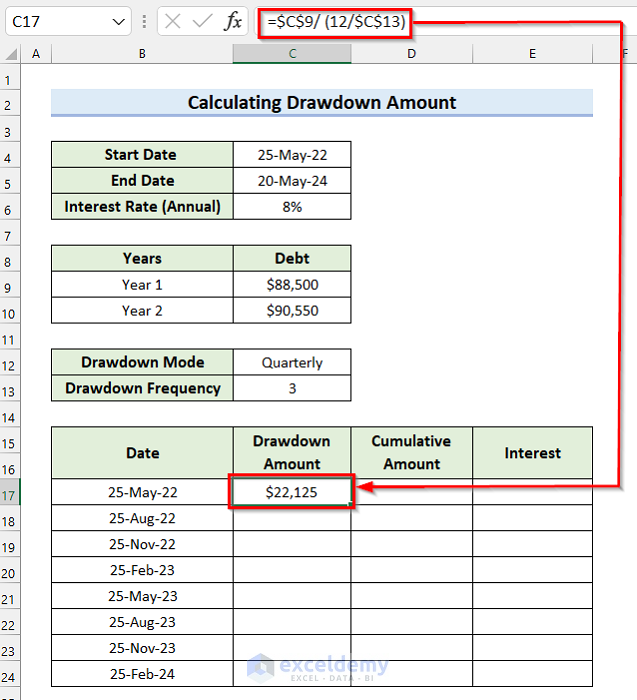
- Drag the Fill Handle down to copy the formula to the remaining cells.
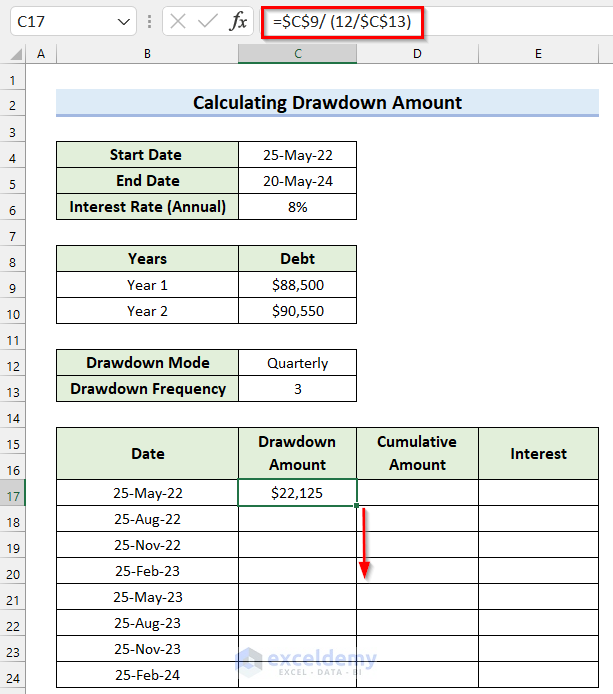
- You can see that we have copied the formula and got the Drawdown Amount for Year 1.
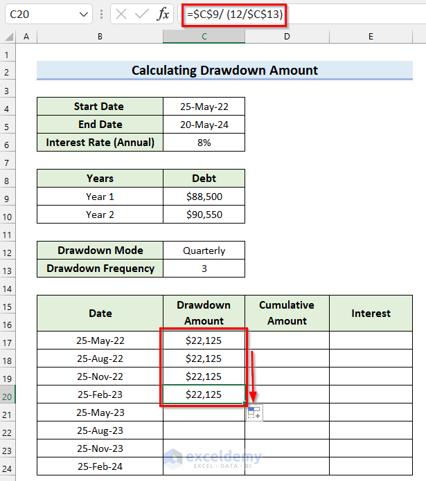
- Select the cell where you want to calculate the Drawdown Amount for Year 2. we have selected cell C21.
- In cell C21, enter the following formula.
=$C$10/(12/$C$13)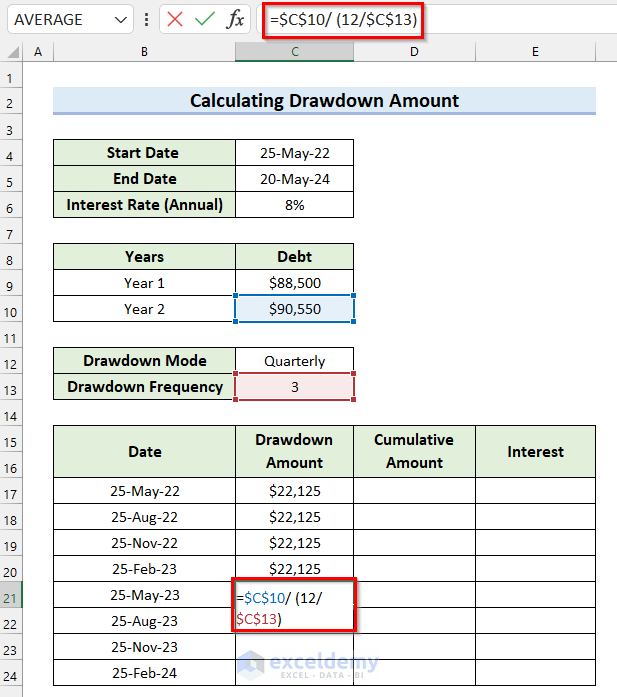
- Press Enter.
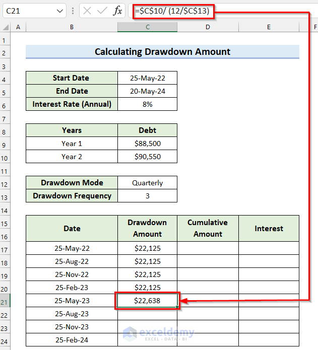
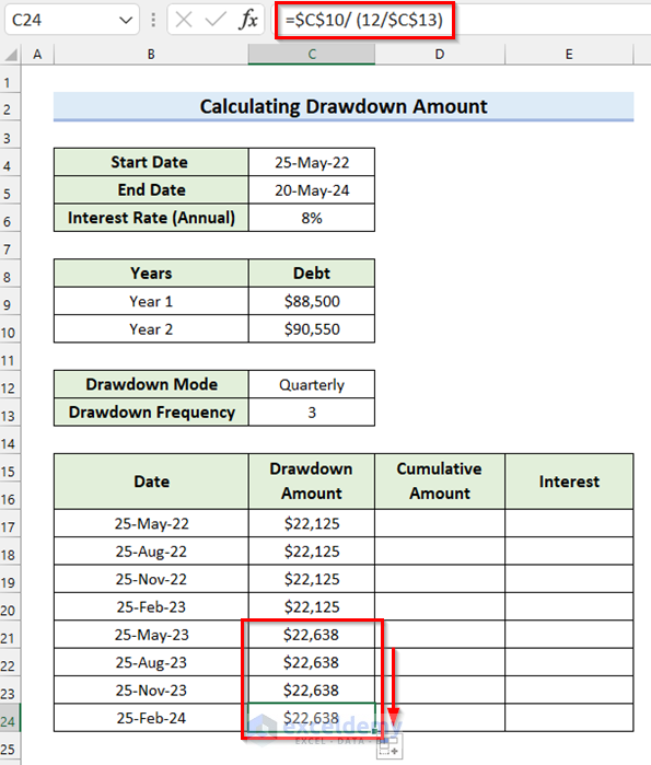
- Drag the Fill Handle down to copy the formula to 3 more cells as the Drawdown Mode is Quarterly.
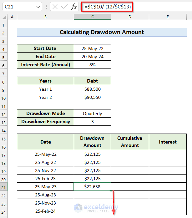
- You can see that we have copied the formula.
Step 5 – Calculate Cumulative Amount
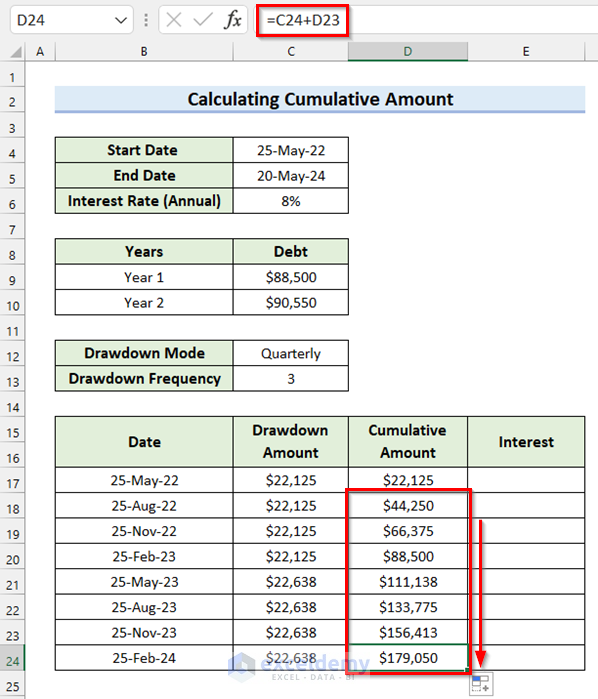
- Select the cell where you want the first Cumulative Amount. we have selected cell D17.
- In cell D17, enter the following formula.
=C17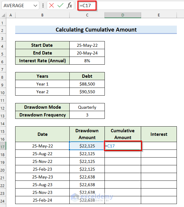
- Press Enter.
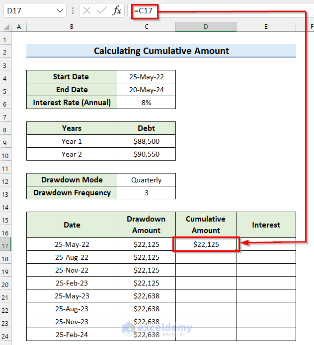
- Select the cell where you want to calculate the next Cumulative Amount.
- Enter the following formula in that selected cell.
=C18+D17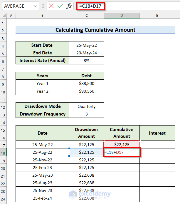
- Press Enter.
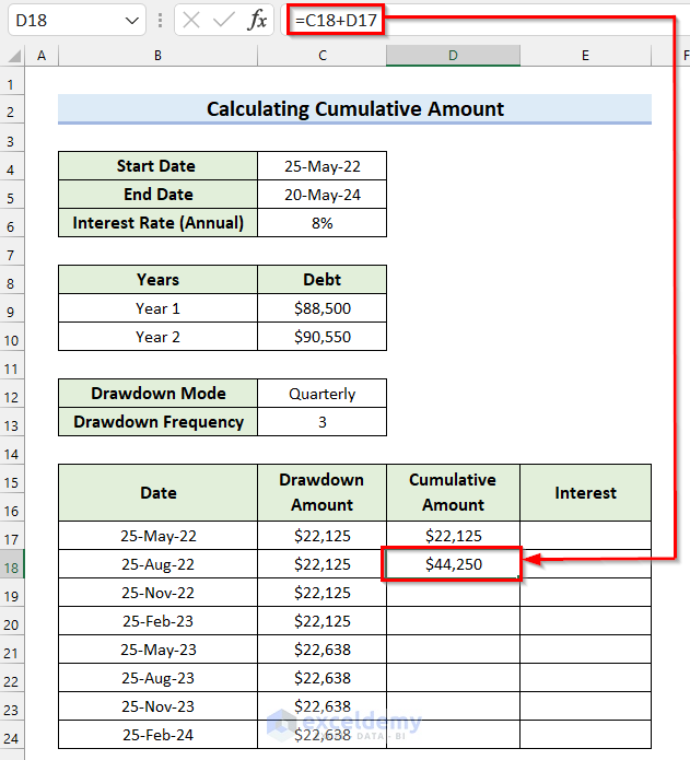
- Use the Fill Handle for the remaining cells.
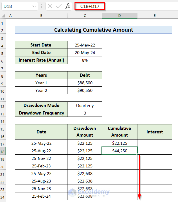
- You can see that we have copied the formula to the other cells and got the Cumulative Amount.
Read More: How to Use Cumulative Interest Formula in Excel
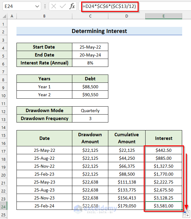
Step 6 – Determine Interest
- Select the cell where you want to calculate the Interest.
- Enter the following formula in that selected cell.
=D17*$C$6*($C$13/12)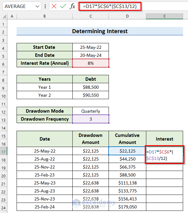
- Press Enter.
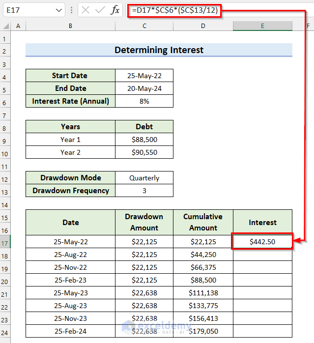
- Use the Fill Handle tool for the remaining cells.
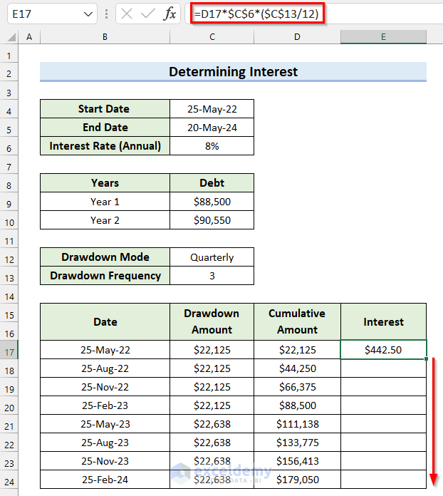
- You can see that we have copied the formula to the other cells and got the Interest.
Step 7 – Calculating Interest During Construction in Excel
- Select the cell where you want to calculate the Interest During Construction. we have selected cell E26.
- In cell E26, enter the following formula.
=SUM(E17:E24)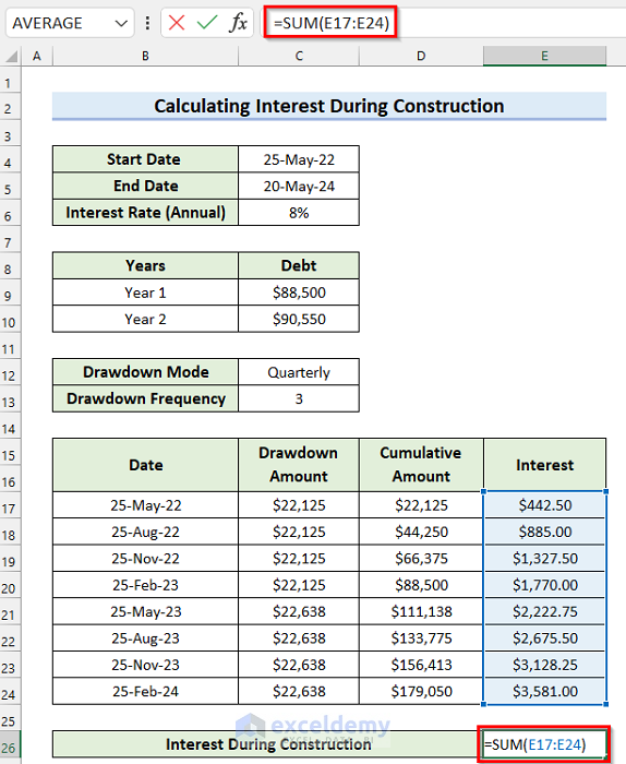
- Press Enter to get the Interest During Construction.
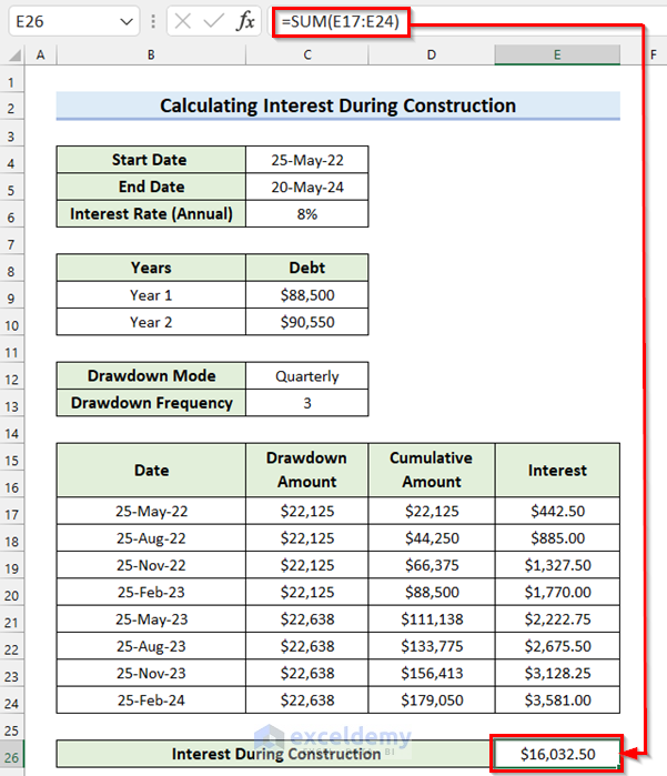
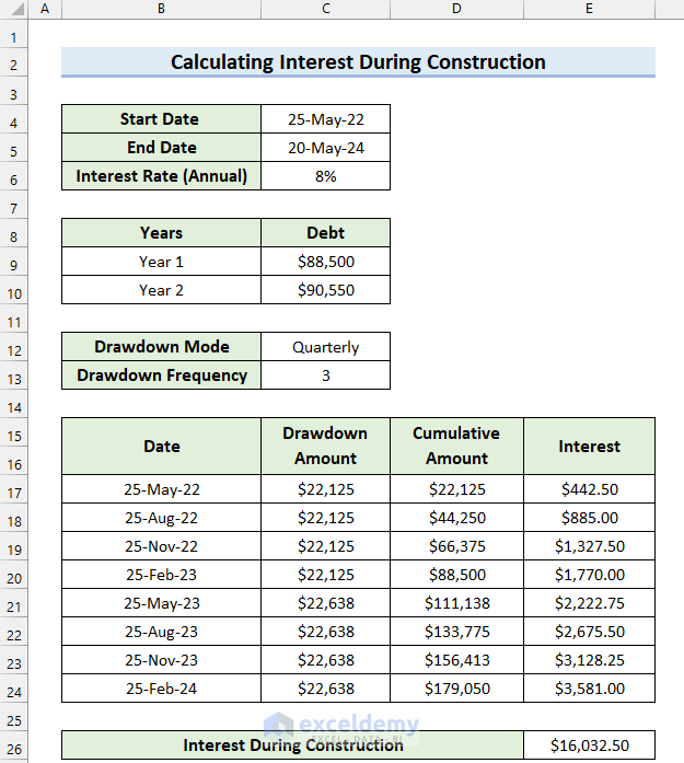
Final Output
In the following image, you can see the final output of the calculation for Interest During Construction.
Download Practice Workbook
Related Articles
- Perform Carried Interest Calculation in Excel
- How to Calculate GPF Interest in Excel
- How to Split Principal and Interest in EMI in Excel
- How to Perform Actual 360 Interest Calculation in Excel
- How to Calculate Daily Interest in Excel
<< Go Back to Excel for Finance | Learn Excel
Get FREE Advanced Excel Exercises with Solutions!

