Keep Row Headings in Excel When Scrolling Without Freeze (2 Ways)

We have selected a dataset with four columns detailing the Product, Brand, Model, and Price. The dataset has 24 rows of data.

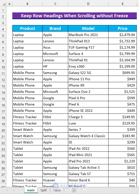
When scrolling down, the headers disappear from view. We will show the headers without using the Freeze Panes feature.

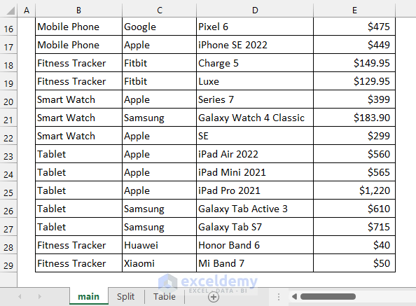
Method 1 – Keeping Row Headings in Excel When Scrolling Without Freeze by Using the Split Pane Feature

Steps:

• Select cell B5.
• From the View tab, select Split.

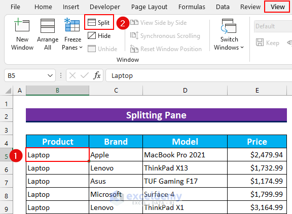
• This will create two gray lines in the dataset. These lines indicate the Split feature is turned on.

• We can scroll down from row 5 and the row headings will still be visible in Excel.

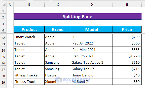
• However, we cannot see any other Sheets inside the Workbook. To make them appear again, the Split feature needs to be turned off. Use the same command to do so.

Read More: How to Make a Row Header in Excel

Method 2 – Creating a Table to Keep the Row Headings When Scrolling Without Freeze

Steps:

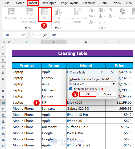
• Select anywhere inside the dataset. We have selected cell C10.
• From the Insert tab, select Table.
• This will make the Create Table dialog box pop up.
• Check if the data range is correct and make sure the “My table has headers” option is selected.
• Press OK.

• This will convert the dataset into a table and we can see the filter arrows or buttons in the row headings.

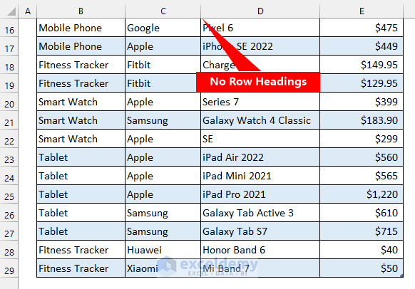
• If we scroll down, the row headings are not visible.

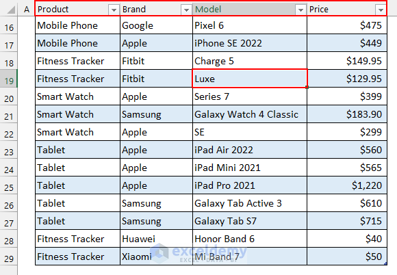
• When we click on a cell inside the table, the row of headings appeared in place of column header letters.

Read More: How to Create a Double Row Header in Excel

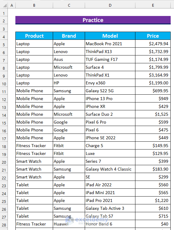
Practice Section

We have added a practice dataset for each method in the Excel file.

Download the Practice Workbook

Related Articles 

• How to Make First Row as Header in Excel
• How to Make Multiple Sortable Headings in Excel
• How to Hide Row and Column Heading in Excel

<< Go Back to Rows and Columns Headings | Rows and Columns in Excel | Learn Excel