Removing duplicates in Excel means keeping the first instance of a value in a range and removing all the other instances. In this Excel tutorial, we will discuss how to remove duplicates in Excel with different tools and functions.
Suppose we have the dataset below containing the Employee ID, Employee Name, Joining Year, and Salary of some employees. There are some duplicate rows. In the animation below, we remove them using the Remove Duplicates command.
This Excel tutorial covers:
- Use of the Remove Duplicates command on single and multiple columns.
- Removal of duplicate rows from a Table with the Remove Duplicates command.
- Using the Advanced filter to remove duplicates.
- Using the UNIQUE function to return only unique values.
- Removal of duplicates except the first instances with the IF-COUNTIF formula.
- Application of Excel formulas and the Filter tool to remove duplicates.
- Removal of duplicates based on criteria with the Advanced Filter tool.
- Use of Power Query for removing duplicates.
- Application of a VBA Macro to remove duplicates from any selection.
⏷1. Using Remove Duplicates Command to Erase Duplicates
⏵1.1. From a Single Column
⏵1.2. Across Multiple Columns
⏷2. Removing Duplicate Rows From Excel Table
⏷3. Removing Duplicate Rows Based on Multiple Columns
⏷4. Applying UNIQUE Function to Remove Duplication
⏷5. Removing Duplicates But Keeping 1st Instance Only
⏷6. Using Formula and Filter Tool to Remove Duplicates
⏷7. Removing Duplicates Based on Criteria
⏷8. Apply VBA Macro to Remove Duplicates
⏷9. Using Power Query Tool to Remove Duplicates
⏷Undo Remove Duplicates
⏷Hide Duplicate Values Instead of Removing Them
⏷Possible Reasons If You Can’t Remove Duplicates
Method 1 – Using the Remove Duplicates Command to Erase Duplicates in Excel
The Remove Duplicates command is the built-in veteran Excel tool to erase duplicate instances. It can be used for removing duplicates from both single and multiple columns.
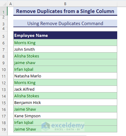
1.1 – From a Single Column
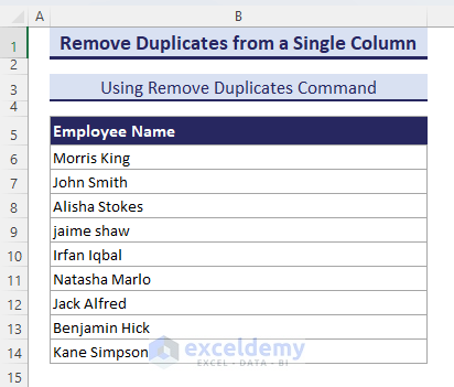
In the image below, we have a list of Employee Names. We will find duplicates and remove them with the Remove Duplicates command.
Steps:
- Find and highlight duplicates with the Conditional Formatting tool.
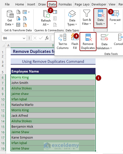
- Select the range B6:B19 and click as follows: Data => Data Tools => Remove Duplicates.
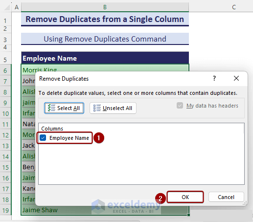
The Remove Duplicates dialog box will appear.
- Check Employee Name => Click OK.
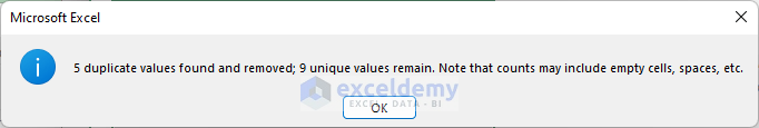
A pop-up dialog box will be visible saying 5 duplicate values found and removed.
- Click OK.
We obtain only unique values, having removed all the duplicates from the list.
Keyboard Shortcut to Remove Duplicates
We can also use a keyboard shortcut to remove duplicates in Excel:
- Press the Alt + A + M keys sequentially to open the Remove Duplicates dialog box.
- Check Employee Name => Click OK.
A list of unique values is returned.
1.2 – Across Multiple Columns
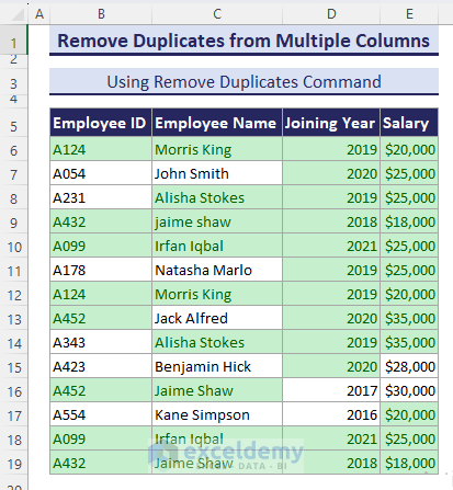
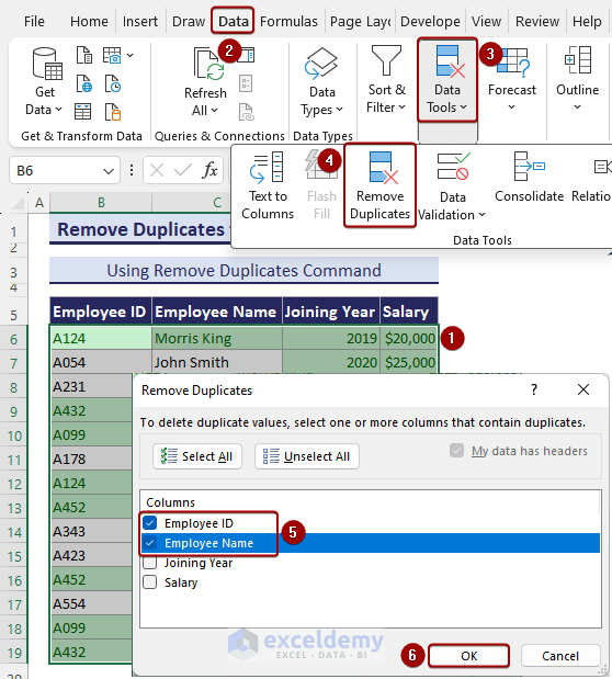
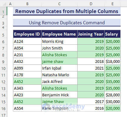
Now we will remove duplicates based on two or multiple columns using Excel’s Remove Duplicates command. First, we will highlight duplicate rows with the Conditional Formatting tool. As in the below image, the 6th, 9th, 10th,12th, 18th, and 19th rows are duplicates. We will remove these duplicate rows based on Employee ID and Employee Name.
- Like before, highlight the duplicate rows with the Conditional Formatting tool.
- Select the range B6:E19 and go to Data => Data Tools => Remove Duplicates.
- In the Remove Duplicates dialog box, check Employee ID and Employee Name => Click OK.
We have unique rows, having removed the duplicate rows.
Method 2 – Removing Duplicate Rows From an Excel Table
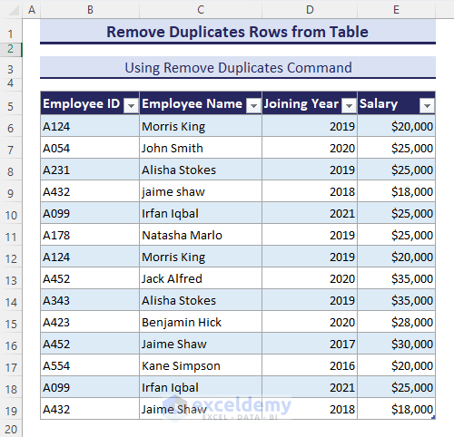
Now we’ll remove duplicate rows from an Excel Table using the Remove Duplicates command. The Remove Duplicates command is also visible in the Table Design tab when you select the table. Below, we have a dataset in a table format containing duplicates. Let’s remove them.
Steps:
- Select the table and go to Table Design => Remove Duplicates.
The Remove Duplicates dialog box will appear.
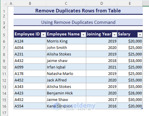
- Check Employee ID and Employee Name => Click OK.

All the duplicate rows will be removed from the table. For example, the 2nd instance of the Employee ID containing A124 & Employee Name with Morris King has been removed.
Method 3 – Removing Duplicate Rows Based on Multiple Columns
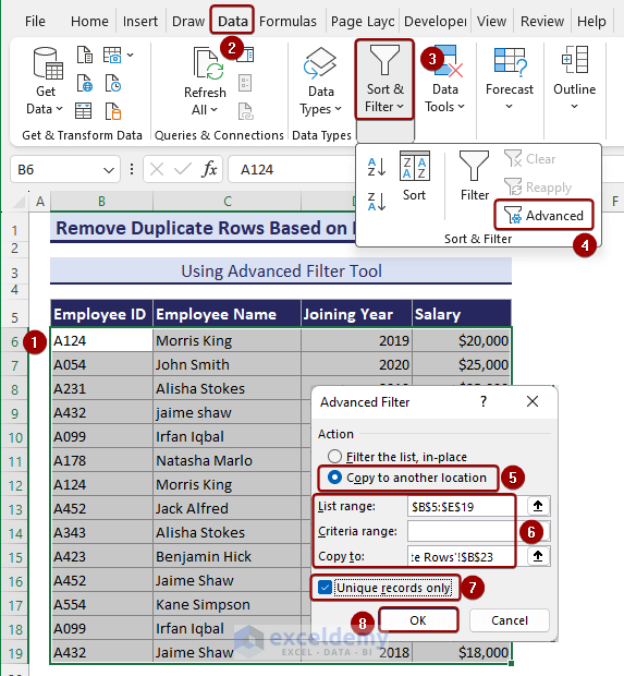
In this method, we’ll remove duplicate rows based on two or more columns using the Excel Advanced Filter tool, which is used to find data that meets multiple complex criteria.
Steps:
- Select the range B6:E19 and click as follows: Data => Sort & Filter => Advanced.
The Advanced Filter dialog box will appear.
- Select Copy to another location from the Action field.
- Select List range $B$5:$E$19, and output location $B$23.
- Check the Unique records only option.
- Click OK.
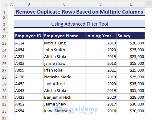
All the filtered unique data will show in the range B23:E33.
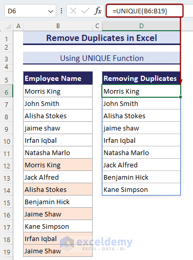
Method 4 – Using the UNIQUE Function to Remove Duplicates
By applying the UNIQUE function, we can retrieve unique values and remove any duplicates in Excel. The UNIQUE function keeps only the first instance and ignores the rest of a dataset. It returns an array.
- Insert the following UNIQUE formula in cell B6:
=UNIQUE(B6:B19)The unique names are returned in an array format.
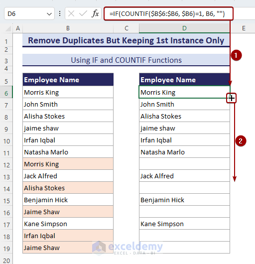
Method 5 – Removing Duplicates in Excel But Keeping the First Instance
We can keep the 1st instance only and remove duplicates by using the IF-COUNTIF functions together in an Excel formula. The COUNTIF function counts the number of instances and the IF function returns the first value only, ignoring further instances. This formula doesn’t return an array, so we can enter it once then use the Fill Handle tool to Autofill an entire column.
- By applying the following IF-COUNTIF formula, we obtain Morris King in cell D6:
=IF(COUNTIF($B$6:$B6, $B6)=1, B6, "")- Use the Fill Handle tool to copy the formula to the cells below.
Method 6 – Using an Excel Formula and the Filter Tool to Remove Duplicates
Now we will remove duplicates with an Excel formula and the Filter tool combined. First, we will find duplicate rows with the IF-COUNTIFS formula. Then we will use the Filter tool to display the duplicate rows only. Finally, the Visible cells only option from the Go To Special dialog box will be used to remove the duplicate rows.
Steps:
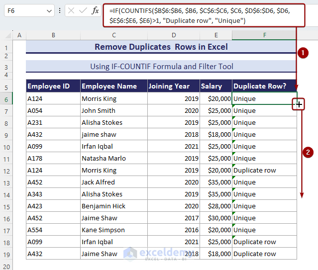
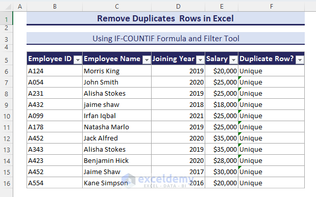
- Apply the following IF-COUNTIFS formula in cell F6 to obtain the output text Unique.
=IF(COUNTIFS($B$6:$B6, $B6, $C$6:$C6, $C6, $D$6:$D6, $D6,$E$6:$E6, $E6)>1, "Duplicate row", "Unique")- Drag down the Fill Handle tool to identify the unique and duplicate rows.
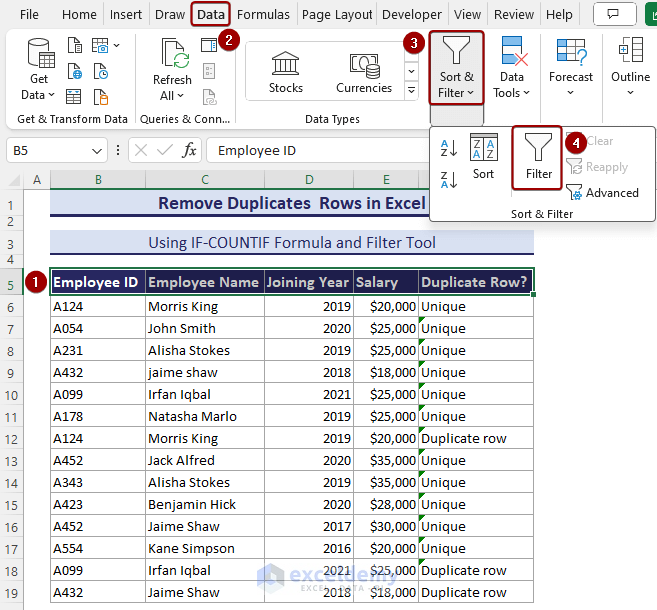
Now, we will select the duplicate rows only with the Filter tool.
- Select the range B5:F5 and click as follows: Data => Sort & Filter => Filter.
- Click on Duplicate Row? => Check Duplicate row => Click OK.
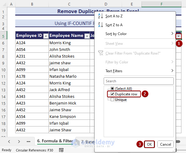
Now we need to select only the duplicate rows.
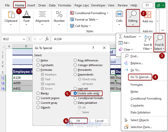
- Go to Home => Editing => Find & Select => Go to Special.
The Go To Special dialog box opens.
- Select the Visible cells only option => Click OK.
All the visible cells will be selected. Now we can delete them.
- Right-click on the Mouse => Select Delete Row from the context menu => Click OK.
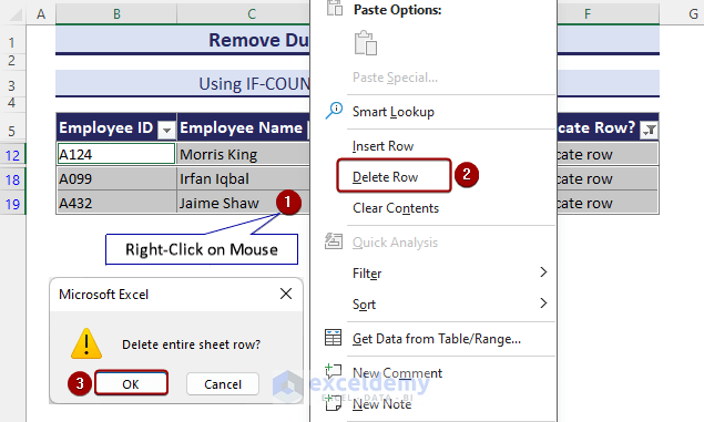
No data will be visible in the spreadsheet.
- Click on the Filter drop-down => Check Unique => Click OK.
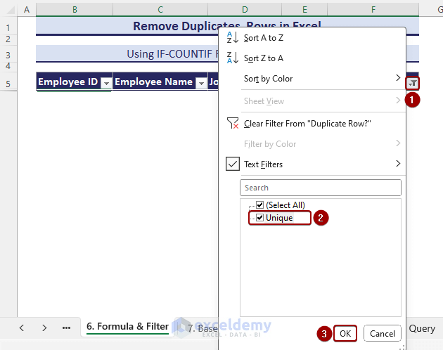
All the unique rows will appear.
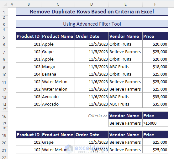
Method 7 – Removing Duplicates Based on Criteria
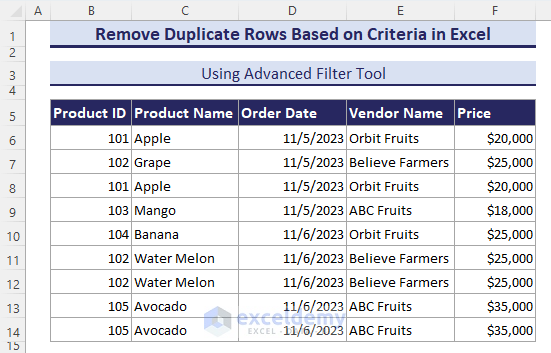
With the Advanced Filter tool, we can remove duplicates based on criteria in Excel. Consider a situation where we import products from some vendors and there are some duplicate rows. We’ll find the duplicates based on 2 criteria: The vendor name will be Believe Farmers & the price will be over $15000.
Steps:
- Select the range B6:F14 and click as follows: Data => Sort & Filter => Advanced.
The Advanced Filter dialog box will appear.
- Select Copy to another location from the Action field.
- Select List range $B$5:$E$19, criteria range $E$16:$F$17, and output location $B$19.
- Check the Unique records only option.
- Click OK.
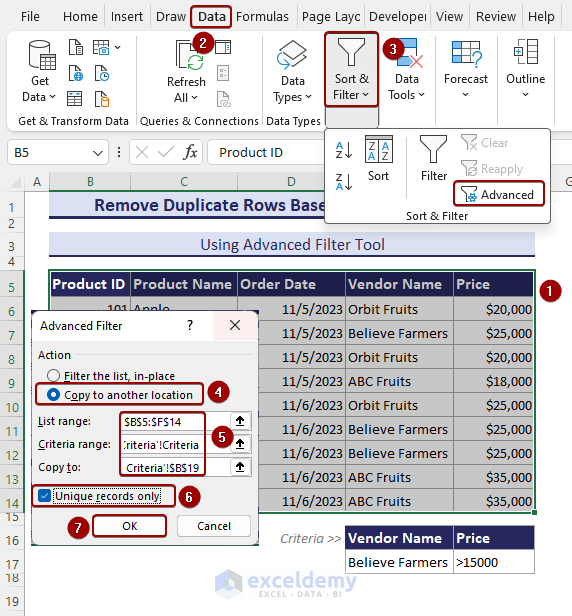
All unique rows containing Believe Farmers and having prices over $15000 will be displayed.
Method 8 – Applying a VBA Macro to Remove Duplicates in Excel
Now we will make a VBA Macro that can be applied anywhere in the worksheet. For a large dataset, it is very useful and saves time. We can develop VBA code to apply to multiple datasets, worksheets, or workbooks at the same time that will remove duplicates automatically.
Steps:
- Enter the following VBA code in the Module and Save the Macro:
Sub Remove_Duplicates_in_Excel()
Dim inp As Range
Set inp = Application.InputBox("Select input range:", Type:=8)
If WorksheetFunction.CountA(inp) > 0 Then
    inp.RemoveDuplicates Columns:=Array(1), Header:=xlNo
Else
    MsgBox "No Data Selected."
End If
End Sub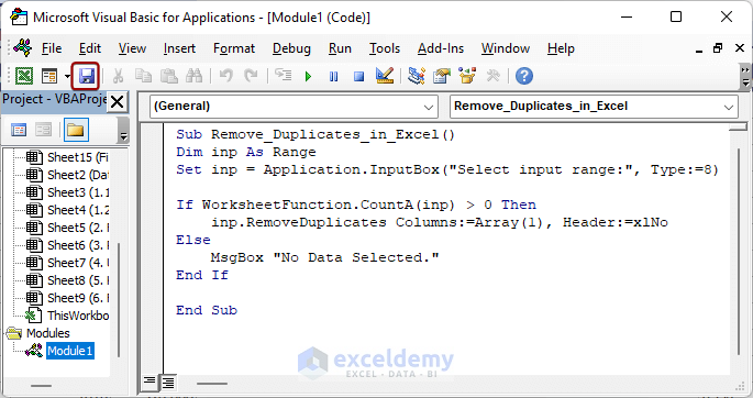
- Select as follows: Developer => Macros => Remove_Duplicates_in_Excel => Run.
- Select the input range.
- Click OK.
The output after removing the duplicates will be returned
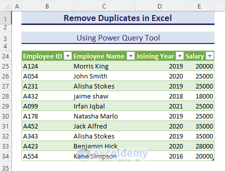
Method 9 – Using the Power Query Tool to Remove Duplicates
We can also use the Power Query tool to remove duplicates in Excel. Power Query allows importing data from external or internal sources. With this approach, we need to perform several steps.
Steps:
- Select the range B5:E19 and go to Data => From Table/Range.
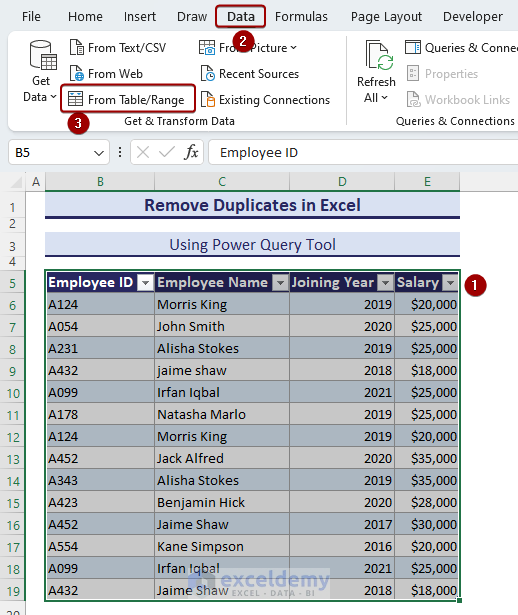
The Power Query Editor will open.
- To find duplicates based on Employee ID, right-click on the 1st column and select the Remove Duplicates command.
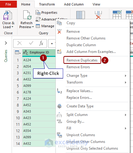
By removing the duplicates, only the unique values will show.
- Select Home => Close & Load drop-down => Close & Load To.
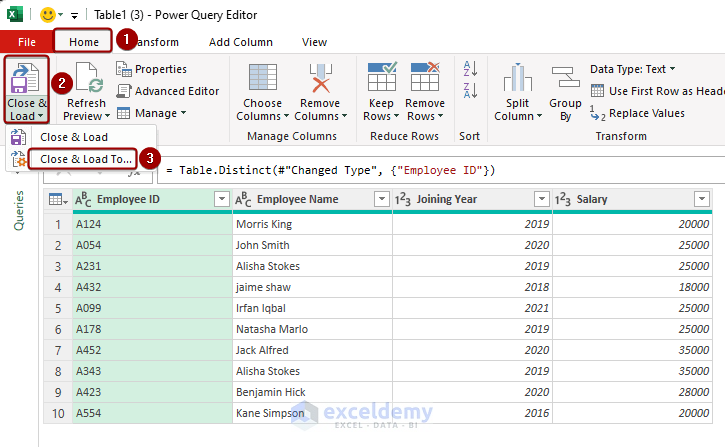
The Import Data dialog box will appear.
- To import the data into a table in the existing worksheet, select Table => Existing worksheet => $B$24 => OK.
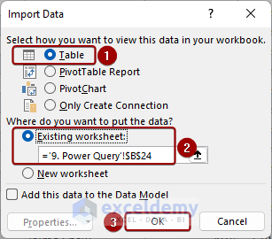
All the unique rows will be inserted into the worksheet, erasing the duplicate rows.
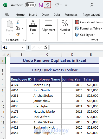
How to Undo Remove Duplicates in Excel?
Suppose, we removed the duplicates, but now we need to undo the remove duplicates operation in Excel.
- Simply click the Undo command from the Quick Access Tool.
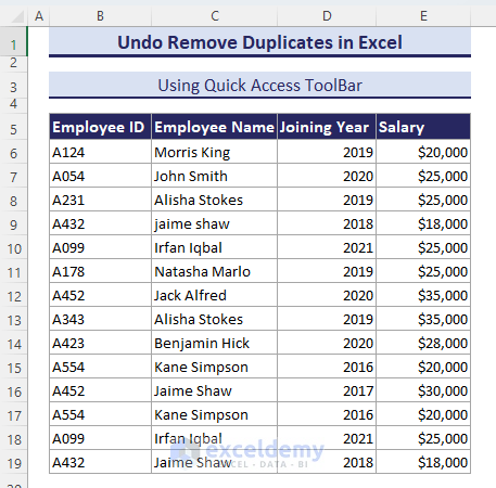
All the data including the duplicates will be shown.
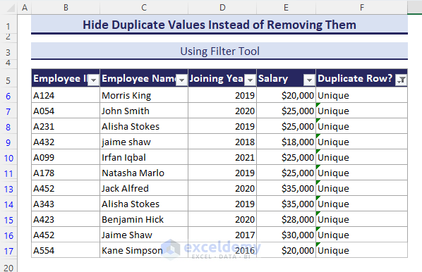
How to Hide Duplicate Values Instead of Removing Them
Instead of removing duplicates, we can hide duplicate values instead with the Filter tool.
Steps:
- Determine the unique and duplicate rows using the IF-COUNTIFS formula in the same way as Method 6:
=IF(COUNTIFS($B$6:$B6, $B6,$C$6:$C6, $C6, $D$6:$D6, $D6, $E$6:$E6, $E6)>1, "Duplicate row", "Unique")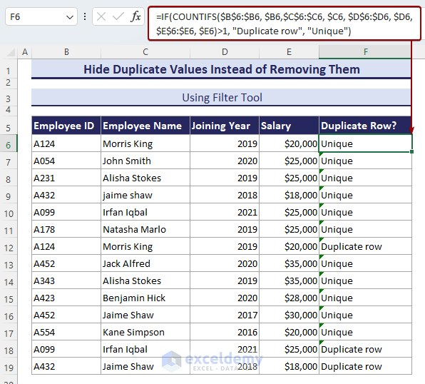
- Select the range B5:F5 and go to Data => Sort & Filter => Filter.
- Click on the Filter drop-down => Check Unique => Click OK.
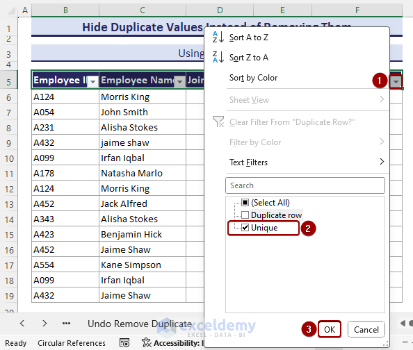 The unique values will be shown, with the duplicates hidden.
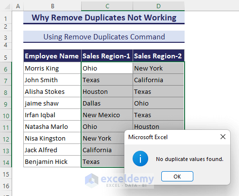
Why Can’t Duplicates Be Removed in Excel Properly?
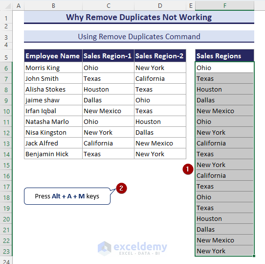
Remove Duplicates tool does not work for two lists. Rather, it treats the cells as duplicate rows. To illustrate, in the image below there are 2 lists of Sales Region.
Issue:
When we select the range B6:D14 and apply the Remove Duplicates command, a pop-up message informs us: No duplicate values found. But the region of Ohio is clearly present in both lists. So, the Remove Duplicate tool is not sufficient to find all duplicate values properly here.
Solution:
- Make a list in column F by copying the data from Sales Regions 1 and 2.
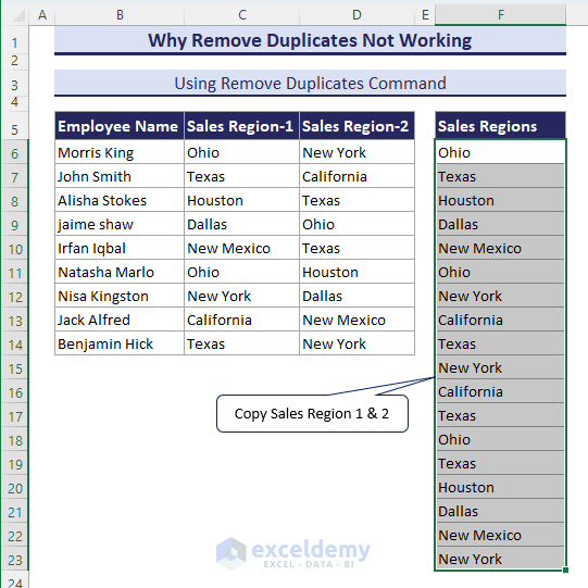
- Select the range F6:F23.
- Press the Alt + A + M keys to apply the Remove Duplicates command.
The Remove Duplicates dialog box pops up.
- Check Sales Regions => Click OK.
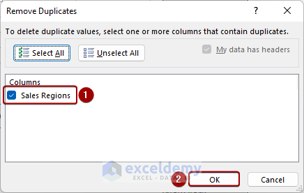
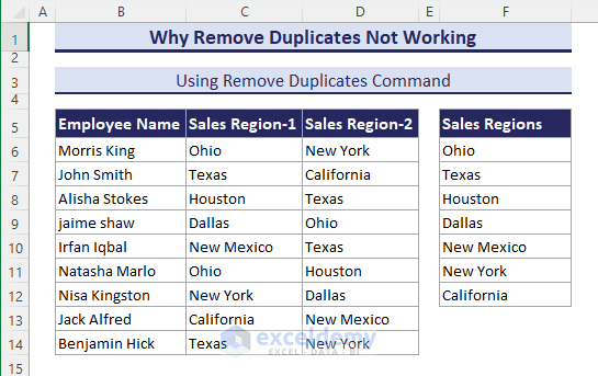
We obtain every Sales Region only once.
Download Practice Workbook
Remove Duplicates in Excel: Knowledge Hub
- How to delete duplicates in excel but keep one
- Remove both duplicates in excel
- How to remove duplicate names in excel
- Excel remove duplicates rows except 1st occurance
- Hide duplicates in excel
- How to remove duplicates in excel using vlookup
- Formula to automatically remove duplicates in excel
- Excel remove duplicate rows
- Excel remove duplicate rows based on one column
- Excel remove duplicates from column
- Excel hide duplicate rows based on one column
<< Go Back to Learn Excel
Get FREE Advanced Excel Exercises with Solutions!
