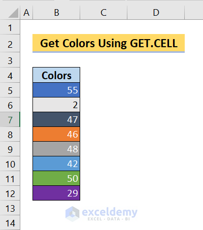
In the following image, you will find an overview of extracting the cell color.
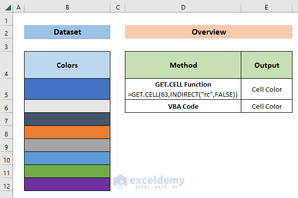
GET.CELL Function in Excel: Overview
The Basic Syntax:
type_num is a number that specifies what type of cell information you want.
You can’t use GET.CELL directly in the worksheet. You need a workaround:
- Go to Formulas and select Name Manager. A Name Manager dialog box will appear.
- Click on New.
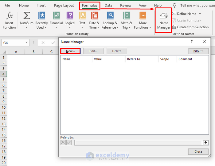
- Enter a name.
- In the Refers to box, use the following:
=GET.CELL(63,INDIRECT("rc",FALSE))As we are working with background colors, we are using 63 in the type_num argument.

- Click OK.
- You can use the GET.CELL property via the name that you have provided.
Introduction to the Color Index and RGB Values in Excel
Excel’s Color Palette has an index of 56 colors which you can use everywhere in your workbook. Each of these colors in the palette is connected with a unique value in the Color Index.
On the other hand, RGB (red, green, and blue) represents the colors on a computer display. The R, G, and B values have a range of decimal numbers from 0 to 255 (256 levels for each color), equivalent to the range of binary numbers from 00000000 to 11111111, or hexadecimal 00 to FF. The total number of available colors is 256 x 256 x 256, or 16,777,216 possible colors.
How to Find the Color Index and RGB Values?
Steps
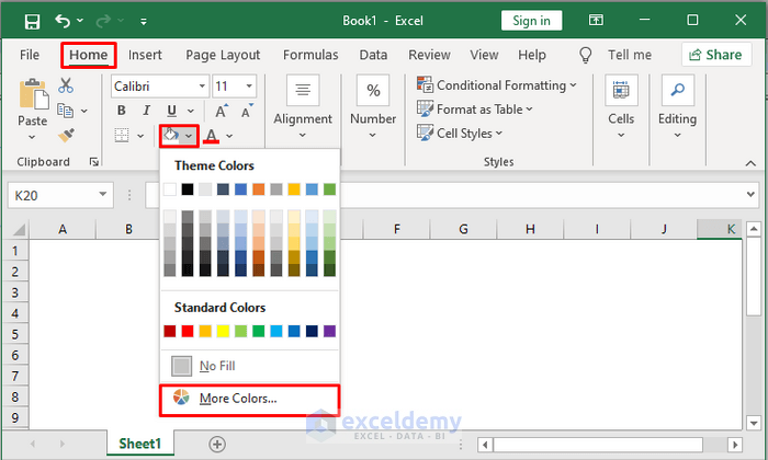
- Go to the Home tab.
- Click on the dropdown Fill Color and select More Colors.
- Click on Custom.
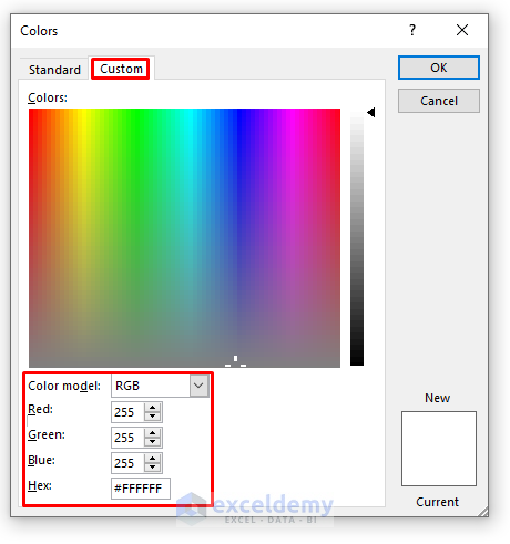
- You’ll find the RGB values of any color in the color model table.
We’ll use a simple dataset where we filled cells of a single column in various colors. We’ll extract the color codes from the cells.
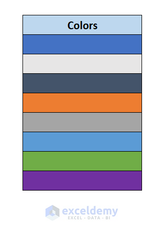
Method 1 – Using the GET.CELL Function to Get the Cell Color in Excel
Steps
- Go to the Formula tab.
- Click on Name Manager. A Name Manager dialog box will appear.
- Click on New.

- Enter a name.
- In the Refers to box, insert the following formula:
=GET.CELL(63,INDIRECT("rc",FALSE))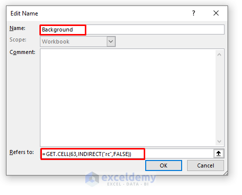
- Click on OK.
- In Cell B5, insert
=Background. If you chose a different name, enter that one.
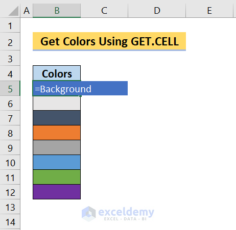
- Press Enter.
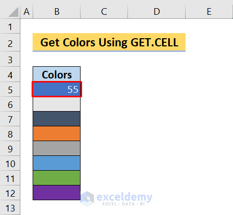
- Repeat for every cell or use AutoFill.
Case 1.1 – Showing the Color Index of a Cell to the Left
Steps
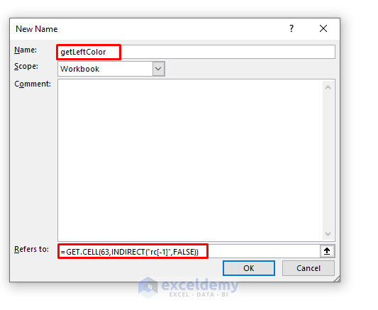
- Go to the Name Manager again. Create a name getLeftColor.
- In the Refers to box, insert the following formula:
=GET.CELL(63,INDIRECT("rc[-1]",FALSE))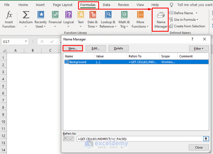
- In Cell E5, enter
=getLeftColor.
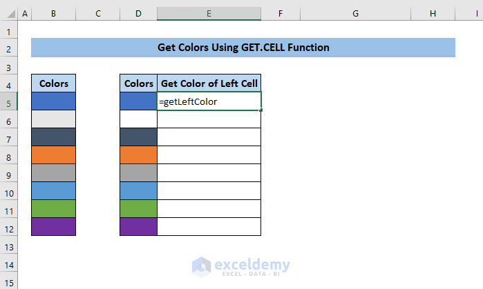
- Press Enter.
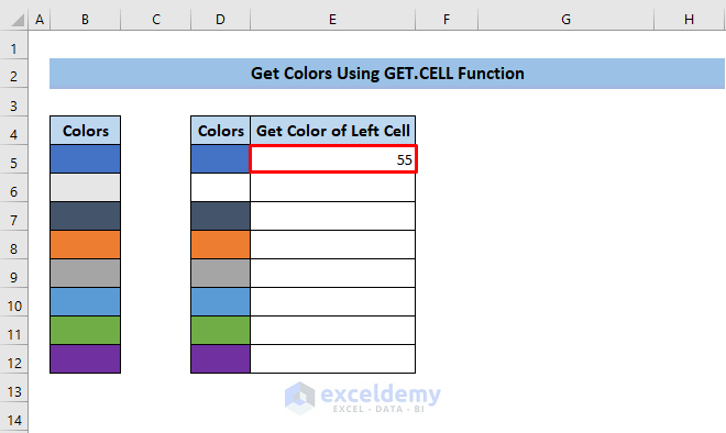
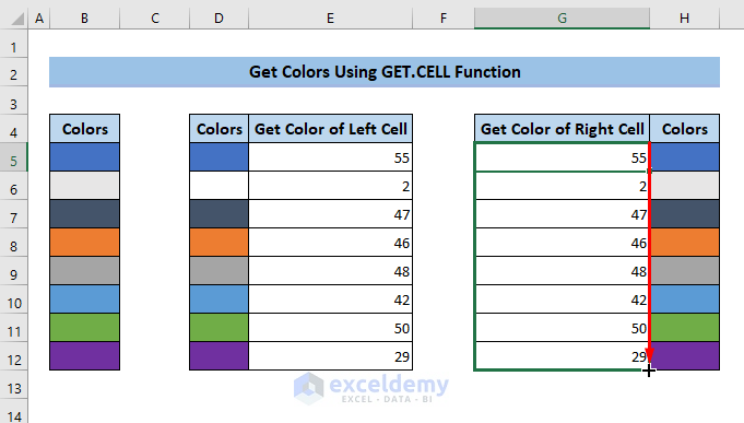
- Drag the Fill Handle icon over the range of cells E6:E12.
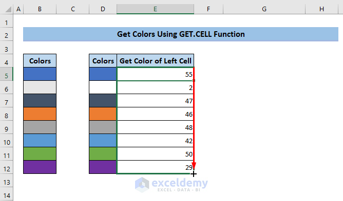
Case 1.2 – Showing the Color Index of the Cell to the Right
Steps
- Go to the Name Manager again. Enter the name getRightColor.
- In the Refers to box, use the following formula:
=GET.CELL(63,INDIRECT("rc[1]",FALSE))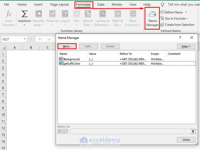
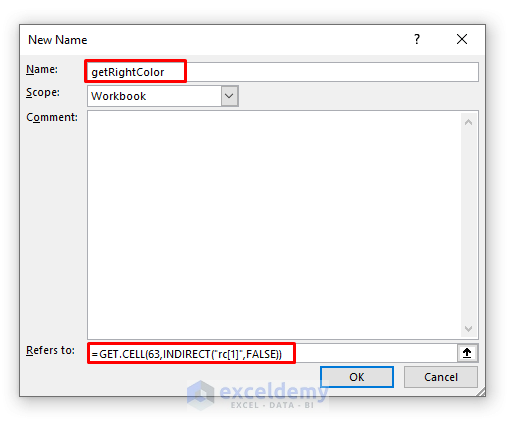
- In Cell G5, use
=getRightColor.
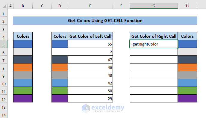
- Press Enter.
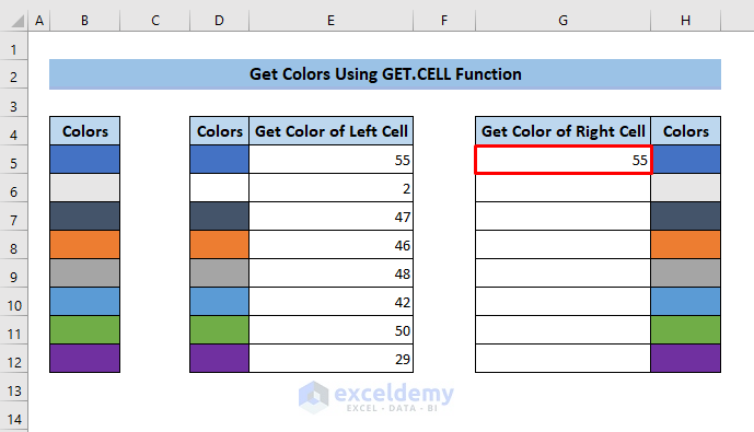
- Drag the Fill Handle icon over the range of cells G6:G12.
Limitation to Use the GET.CELL Function:
If you change the color of the cell, the value won’t change. Press F9 on your keyboard to recalculate it again.
Method 2 – Using VBA Code to Get the Cell Color in Excel
Case 2.1 – VBA Code to Get the Cell Color Index
Steps
- Press Alt + F11 to open the VBA editor.
- Click on Insert and choose Module.

- Insert the following code:
Function ColorIn(color As Range) As Integer
ColorIn = color.Interior.ColorIndex
End Function- Save the file.
- In Cell B5, insert the following formula:
=ColorIn(B5)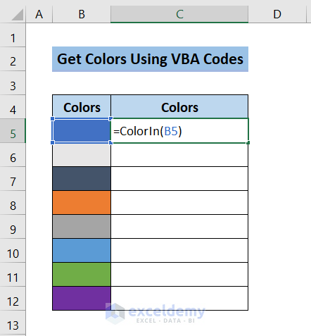
- Press Enter.
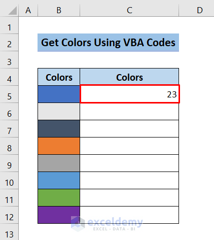
- Drag the Fill Handle icon over the range of cells B6:B12.
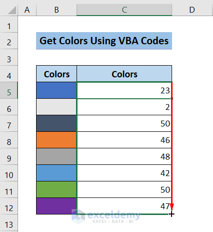
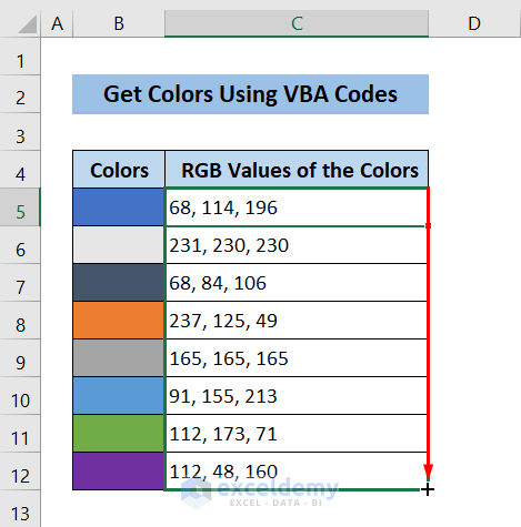
Case 2.2 – VBA Code to Get the RGB Value of Cells
Steps
- Press Alt + F11 to open the VBA editor.
- Click on Insert and select Module.
- Insert the following code:
Function FindColor(cell_range As Range, ByVal Format As String) As Variant
Dim ColorValue As Variant
ColorValue = Cells(cell_range.Row, cell_range.Column).Interior.color
Select Case LCase(Format)
Case "rgb"
FindColor = (ColorValue Mod 256) & ", " & ((ColorValue \ 256) Mod 256) & ", " & (ColorValue \ 65536)
Case Else
FindColor = "Use'RGB' as second argument!"
End Select
End Function- Save the file.
- In Cell B5, use the following formula:
=FindColor(B5,"rgb")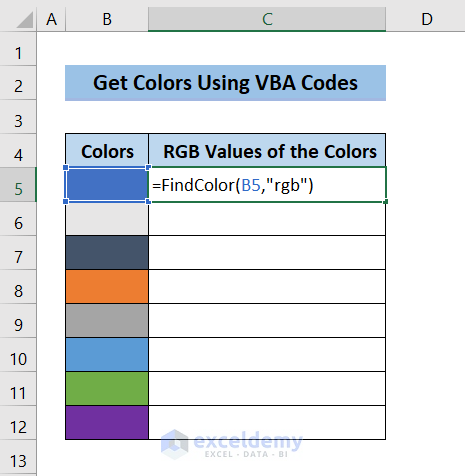
- Press Enter.
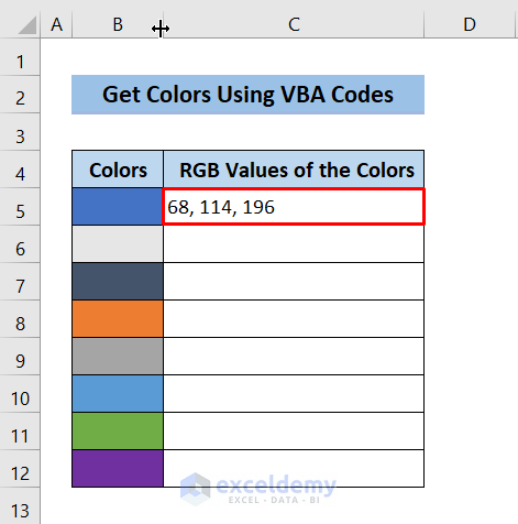
- Drag the Fill Handle icon over the range of cells B6:B12.
Download the Practice Workbook
Excel Get Cell Color: Knowledge Hub
<< Go Back to Excel Cell Format | Learn Excel
Get FREE Advanced Excel Exercises with Solutions!


i rarely saw such bad explanations, i don’t understand anything
for instance, in the downloaded excel file, i cannot see nowhere the function GET.CELL
????
Hi Blump,
We do use Microsoft 365 version to make our documents. If you use older versions of Excel, you may not find it.
By the way, thanks for your feedback.
Thanks.
Hi, good post thanks. I have formatted cells by conditional not manual work, could it be possible to get this background color??
I’m listening!!! 🙂
I really hope there is a way to extract the color information of a conditional formatted cell.
use 38 or 39 in the get.cell function
https://d13ot9o61jdzpp.cloudfront.net/files/Get_Function.pdf
or
https://www.exceldemy.com/excel-formula-based-on-cell-color/
Neither 38, nor 39 works 🙁
To extract color information of conditional formatting cells, you need to follow the steps
1. First, use the conditional formattings in your dataset.
2. Then, click on the Dialog Box Launcher (Small tilted arrow beside Clipboard) from the Clipboard group.
3. After that, click on Clear All from there.
4. Copy the conditionally formatted range.
5. Now, select a new cell where you want to paste your conditional formatting range color only.
6. After that, click on Paste All from the Clipboard group.
7. Now, remove the numbers and only remains the conditional formatting colors.
8. Now, use =Background or =getLeftColor or =getRightColor just like this article, you will get your desired color information.
Try this solution I think you will get your desired result. If you face any more problems, inform us.
https://www.exceldemy.com/excel-formula-based-on-cell-color/
Hello Mark SIMONS and GVG,
Can you please share your Excel dataset with us? Then, we will try our best to provide you with the required solution.
If you have the Indirect address to another file in a cell to the left, you can use this formula instead: =GET.CELL(63,INDIRECT(INDIRECT(“RC[-1]”,FALSE),TRUE))
The indirect address would be ‘[fileName.xlsm]sheetName’!$A$1
Hello, DANIEL DUMITRU!
Thanks for your comment. Appreciate your efforts. Stay connected with us!
Good Luck!
Regards,
Sabrina Ayon
Author, ExcelDemy.
Brilliant!
Very useful!
Thank you!
Hello, Suki Nasoordeen!
Thanks for your appreciation. Stay in touch with ExcelDemy.
Regards
ExcelDemy
Unfortunately this didn’t work. It just shows the formula, not the number
Hello, STEVE C.
Thank you for sharing your problem with us. All the methods shown in the article should work perfectly for Microsoft 365 version. You might be using an older version. That’s why you are facing the problem. So, make sure to activate Microsoft 365 on your PC. Then, you should be able to use these procedures to get the color index.
Do let us know if your problem is solved or not.
Regards,
Sourav Kundu
ExcelDemy
It does not work!
I inserted the VBA script you mention for Index.
Saved the file as excel with macros.
inserted the formula ColorIn(B5) as instructed.
No matter what color I use, it always shows -4142 as a result
Hello Miriam,
Thank you for sharing your problem with us. We are sorry you’re experiencing issues with the Excel VBA script for getting cell color.
Here are a few steps you can take to address the problem:
Please let us know if your problem is solved or not.
Regards,
Bishawajit Chakraborty
ExcelDemy
It does not work with color information of conditional formatting cells, The reply from DURJOY PAUL is not clear, especially step 7
Hello SHIQIANG
Thanks for sharing your problem. Typically, we are unable to perform such tasks in Excel. However, you can try using an Excel VBA Sub-procedure I have developed. It will display all the color indexes of the selected cells in the Immediate Window. The idea works perfectly if background is set manually or only one conditional formatting rule is applied in a cell. You can easily modify the formula for multiple conditional formatting rules based on your needs.
OUTPUT Overview:
Excel VBA Code:
Reach out again if you have any further queries. Hopefully, the idea will help you; good luck.
Regards
Lutfor Rahman Shimanto
Excel & VBA Developer
ExcelDemy
I am using this for a SolidWorks Design Table and it seems to work very well in excel outside of SW. However, once excel is initiated and run from within the SW application, it will not work and just shows #BLOCKED! in the cell?!?! Please help! I’ve gone thru all the settings in the excel trust center, nothing works. I had high hopes for this is exactly what I need, but SW does not allow for VBA due to restrictions.
Hello Steve Zimmermann
Thanks for visiting our blog and sharing your problem. You mentioned that the existing article methods work fine for regular Excel but not when opened inside SolidWorks (SW). Instead of showing the cell color, you get a #BLOCKED! Error; it shows up when a required resource can not be accessible.
It seems there are compatibility issues between VBA functionalities and SolidWorks. When Excel is opened by other applications like SolidWorks, some features and functionalities may not be available. As a result, when some resources are unavailable, they show #BLOCKED!
To overcome your situation, you can check the settings related to external scripting. You can also reach out to the SolidWorks community forum. Providing a solution without glancing at your file and being remote is very tough. I hope these ideas will help you; good luck.
Regards
Lutfor Rahman Shimanto
ExcelDemy
Thanks a lot, the first option really helped.
Hello Sviat,
You are most welcome. Thanks for your feedback! Glad to hear that first option really worked for you. Keep exploring Excel with ExcelDemy!
Regards
ExcelDemy