How to Round to Significant Figures in Excel: 2 Suitable Methods

Method 1 – Using Excel Formula Round to Significant Figures

1.1 Combining ROUND, INT, LOG10 & ABS Functions

Steps:

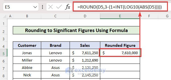
• Paste the following formula into cell E5 to round the value of cell D5 to 3 significant digits.

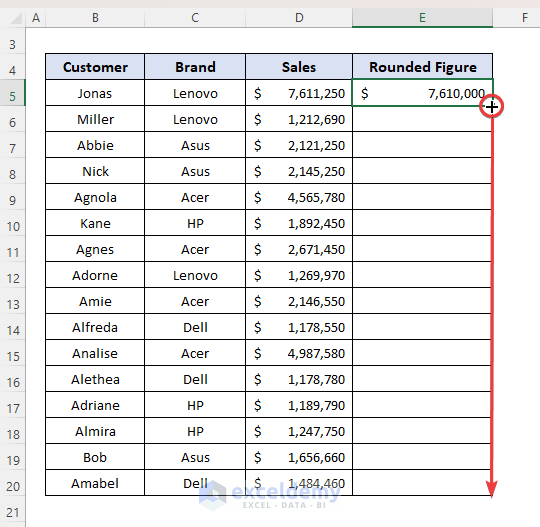
• Drag the Fill Handle icon to paste the formula to the other cells of the column, or use Excel keyboard shortcuts Ctrl+C and Ctrl+V to copy and paste.

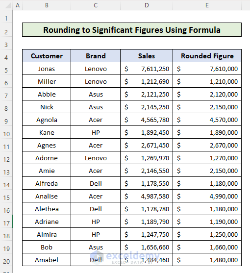
• Get the values of the Sales column rounded to 2 significant.

1.2 Using Excel Formula with ROUND, INT & LOG10 Functions to Round to Significant Figures

Steps:

• Create a cell to take the input of significant figures.

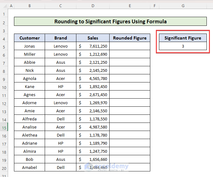
• Paste the following formula into cell E5:

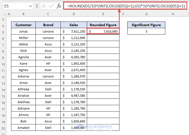
• Drag the fill handle icon to the last cell of the column and get the column filled with the output of the same formula.
• The Sales Column values are rounded to 3 significant figures.

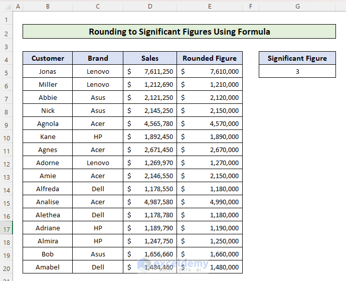
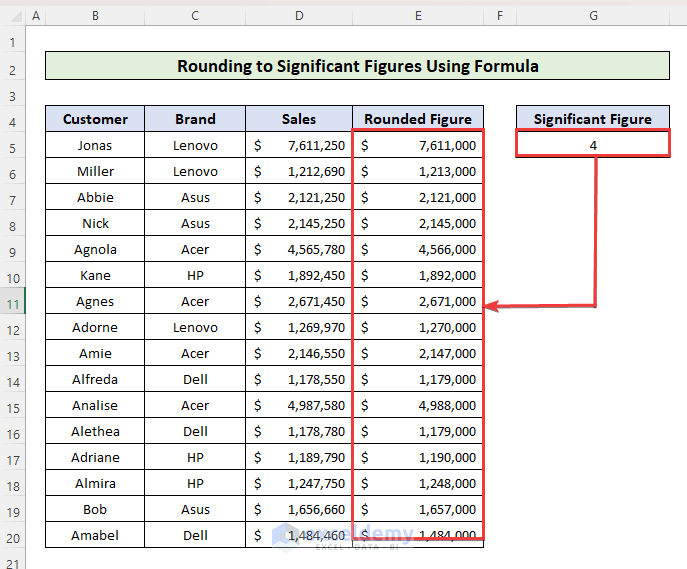
• Change the value of the significant figures in cell G5 to 4 and you will see the Rounded Figure column is changed automatically to 4 significant figures.

Method 2 – Applying VBA Custom Function to Round to Significant Figures

Steps:

• Go to the top ribbon, press on the Developer, and then press on the Visual Basic option from the menu.

Use ALT + F11 to open the ‘Microsoft Visual Basic for Applications’ window if you don’t have the Developer tab added.

• A window named “Microsoft Visual Basic for Applications” will appear. From the top menu bar, press on the “Insert” a menu will appear. Select the “Module’” option.

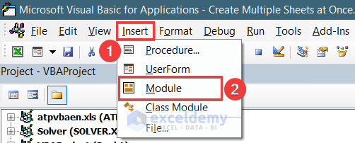
• A new “Module” window will appear, and Paste this VBA code into the box.

Function ROUNDSIGNIFICANT(Value As Variant, Digits As Variant)
Dim exp As Double
If IsNumeric(Value) And IsNumeric(Digits) Then
If Digits < 1 Then
' Please Insert the  " #NUM "  error
ROUNDSIGNIFICANT = CVErr(xlErrNum)
Else
If Value <> 0 Then
exp = Int(Log(Abs(Value)) / Log(10#))
Else
exp = 0
End If
ROUNDSIGNIFICANT = WorksheetFunction.Round(Value, _
Digits - (1 + exp))
End If
Else
' Please Insert the  " #N/A "  error
ROUNDSIGNIFICANT = CVErr(xlErrNA)
End If
End Function

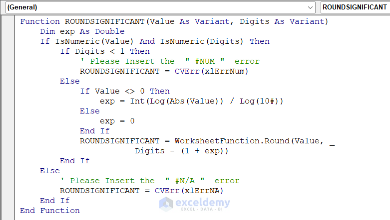
• After inserting the code in the module, come back to the worksheet. Use a new function named ROUNDSIGNIFICANT to round values to significant figures in Excel.
• Paste this formula into cell E5 and it will return the rounded values.

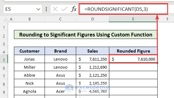
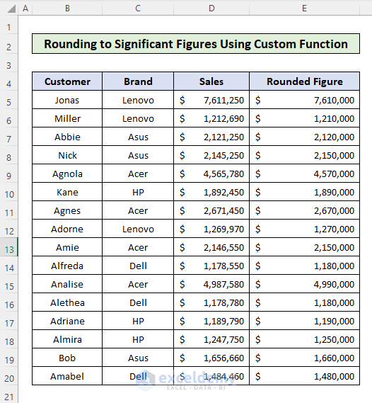
• Drag the Fill Handle icon to paste the used formula respectively to the other cells of the column or use Ctrl+C and Ctrl+V to copy and paste.

Things to Remember

• Using the first formula shown in this article, If you want to change the number of significant figures then you have to change the formula in each cell.
• But using the 2nd formula, to change the number of significant figures, you have to insert the value in the G5 cell.
• While using the VBA code, you don’t have to run the code. Just paste it into the module code and come to the Excel worksheet.

Download Practice Workbook

You can download the practice workbook from here:

<< Go Back to Rounding in Excel | Number Format | Learn Excel