How to Remove Sort in Excel (3 Easy Methods)

Method 1 – Use the Conventional Undo Command to Remove Sort in Excel

To demonstrate this method, we will use the following dataset. We have filter buttons in the header cells. We will sort the data, then remove the sorting.

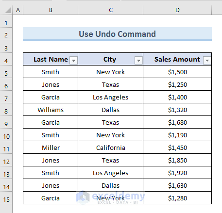
Steps:

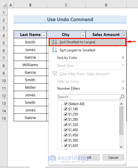
• Click on the filter button of the header cell D4.
• Select Sort Smallest to Largest from the available options.

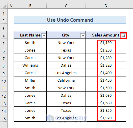
• We can see the sorting icon in cell D4. The value in the Sales Amount column is also sorted from smallest to largest value.

• Press Ctrl + Z.
• We get back to the original dataset without the sort.

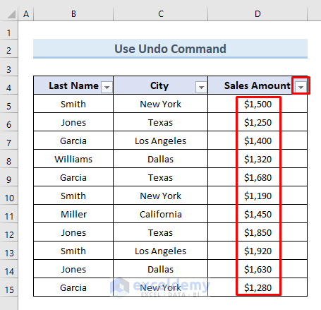
NOTE: The undo command can only undo an immediate action. If you close the worksheet and open it later, you will not be able to remove sorting with the Ctrl + Z command.

Read More: How to Undo Sort in Excel

Method 2 – Remove Sort in Excel Using the ‘Sort & Filter’ Option

We will use the dataset of our previous example to demonstrate this method.

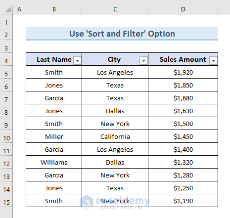
Steps:

• Click on the filter button of the header cell D4.
• Select the option Sort Largest to Smallest.

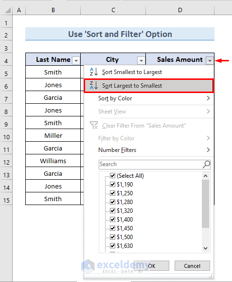
• The sorting icon is in cell D4. We get the sorted values of the “Sales Amount” column from largest to smallest.

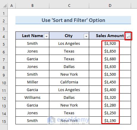
• Go to the Home tab.

• From the Editing section of the Home tab, open the Sort & Filter drop-down.
• Select the option Clear from the drop-down.

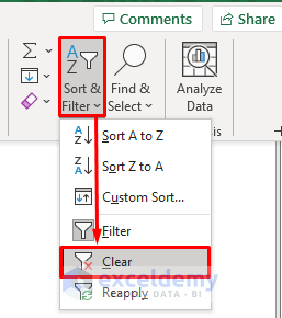
• The sorting icon from the header cell D4 was removed.

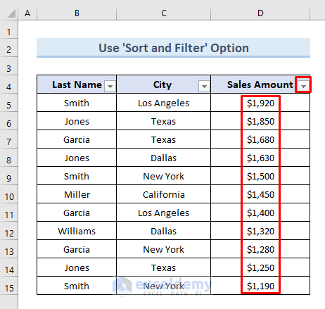
NOTE: The Sort & Filter option only removes the sorting icon. This option does not restore the dataset to the original version.

Read More: How to Sort by Ascending Order in Excel

Method 3 – Insert an Index Column to Remove Sort in Excel

With an additional column, we can always tell the status of the dataset if it is sorted or not. We have the following dataset in table form, and we will insert an index column to remove the sort of this dataset.

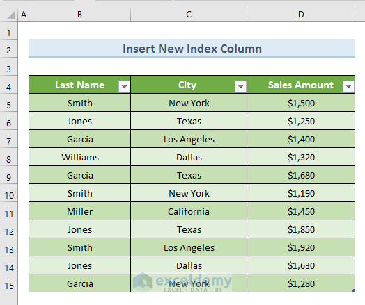
Steps:

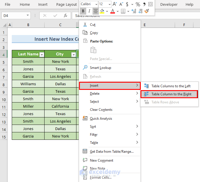
• Right-click on any cell in the Sales Amount.
• Go to the Insert option and select Table Column to the Right.

• We can see an additional column on the right side of the column “Sales Amount”.

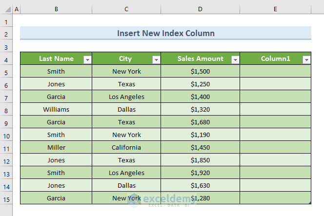
• Rename the additional column to New Index.

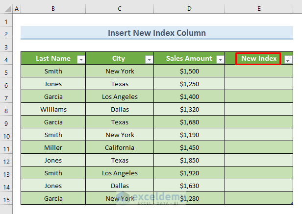
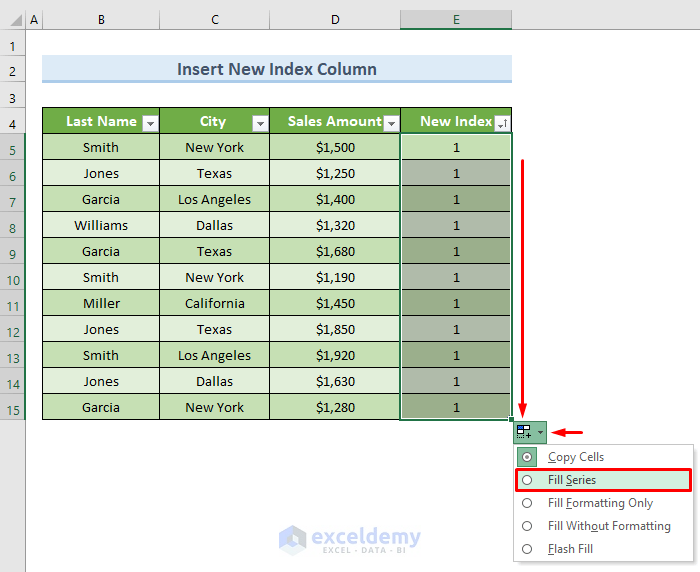
• Insert value 1 in cell E5. Select the cell and drag the Fill Handle tool to the end of the column.
• From the dropdown of the right bottom corner, select the option Fill Series.

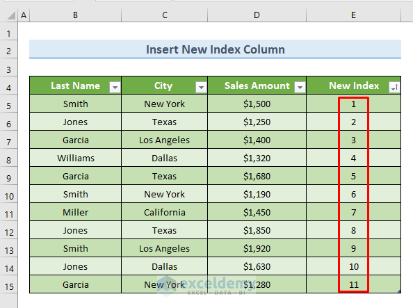
• We get a series of index numbers in the New Index.

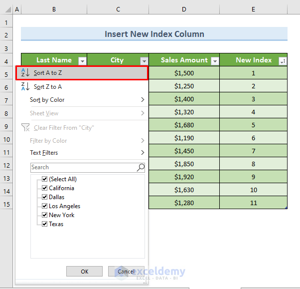
• Click on the filter icon in cell C4. Sort the column City by using the option Sort A to Z.

• The values of column “City” are sorted alphabetically from A to Z. The values of the column New Index are also sorted with the column City.

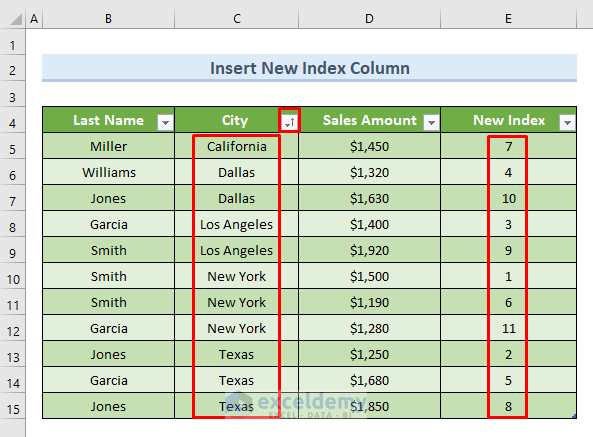
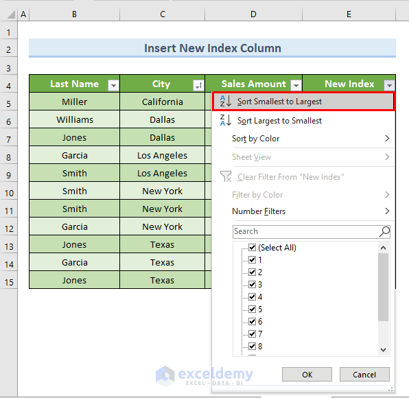
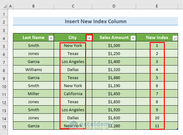
• The New Index column keeps track of whether our data is sorted. To remove the sorting from our dataset, sort the New Index column by Smallest to Largest.

• This effectively undoes the sort for City.

NOTE: If you are filtering data using data range, the filtering option will not be available in the newly inserted column. You have to apply the filtering option again in the newly inserted column.

Read More: How to Remove Sort by Color in Excel

Download Practice Workbook

You can download the practice workbook from here.

Related Articles

• How to Add Sort Button in Excel
• How to Use Excel Shortcut to Sort Data
• How to Sort Data in Excel Using Formula
• How to Sort Data in Alphabetical Order in Excel
• How to Sort Alphanumeric Data in Excel
• Excel Sort and Ignore Blanks
• How to Sort by Color in Excel
• How to Sort Data by Value in Excel

Remove Sort in Excel: Knowledge Hub

• How to Undo Sort in Excel
• How to Remove Sort by Color in Excel

<< Go Back to Sort in Excel | Learn Excel