Method 1 – Insert Arrows Manually from the Symbol Dialog Box
The easiest way to insert arrows is from the Symbol option. Suppose we have the sales amount of some products for January and February.
- Calculate the differences between January and February in column E using the following formula.
=D5-C5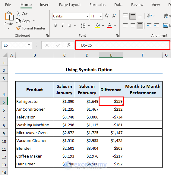
- Go to the Insert tab >> Select Symbol.
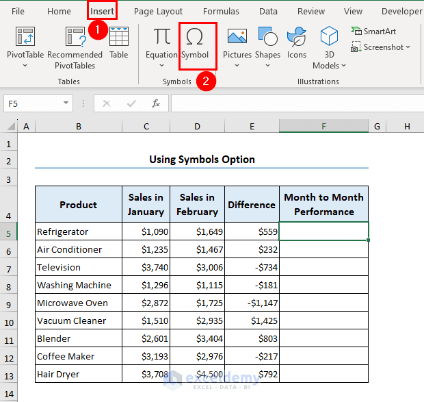
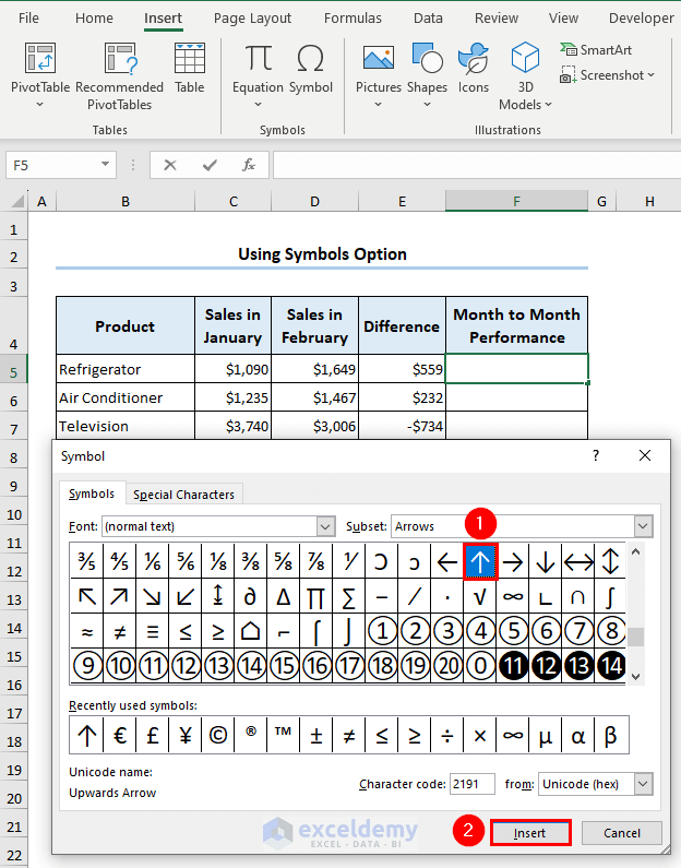
- Insert the arrows based on the sales value.
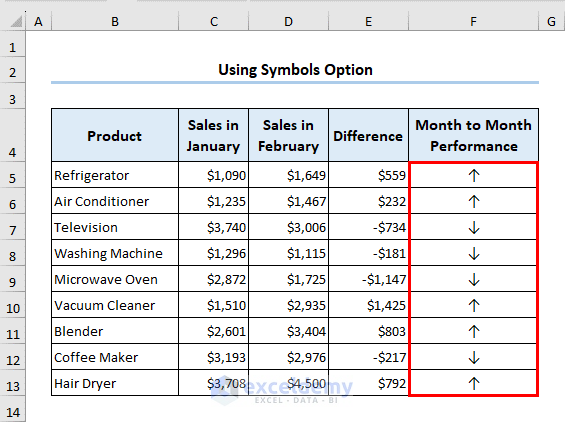
- For a positive difference, paste an upward arrow (↑); for a negative one, we will paste a downward arrow (↓).
- For example, refrigerator sales increased by $559 in February, so we will have an upward arrow in F5.
- Insert the arrows in the rest of the cells.
Method 2 – Use Copy and Paste Operations to Insert Arrows in Excel
- Insert arrows from the list of symbols. These will be placed separately from the main dataset.
- We inserted the upward arrow (↑) in cell H5 and the downward arrow (↓) in cell H6.
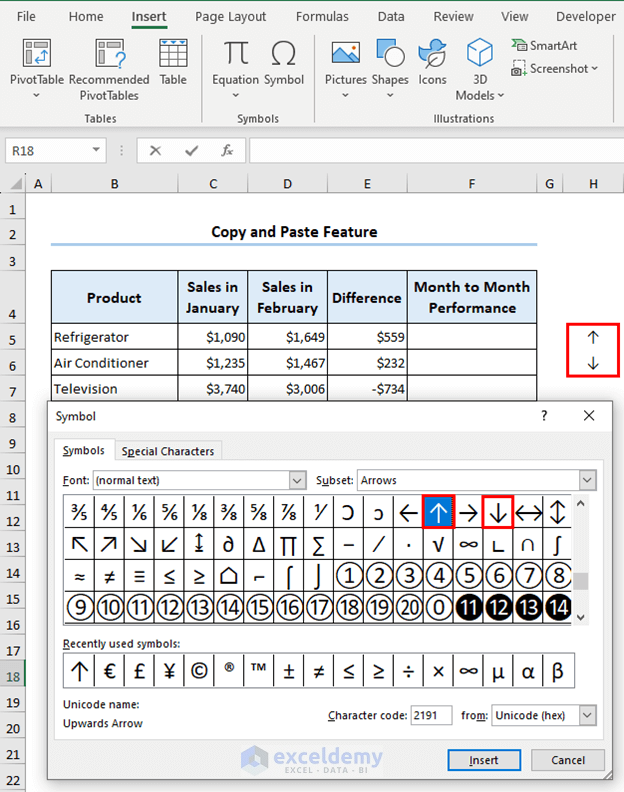
- Copy the symbols and paste them into the respective cells.
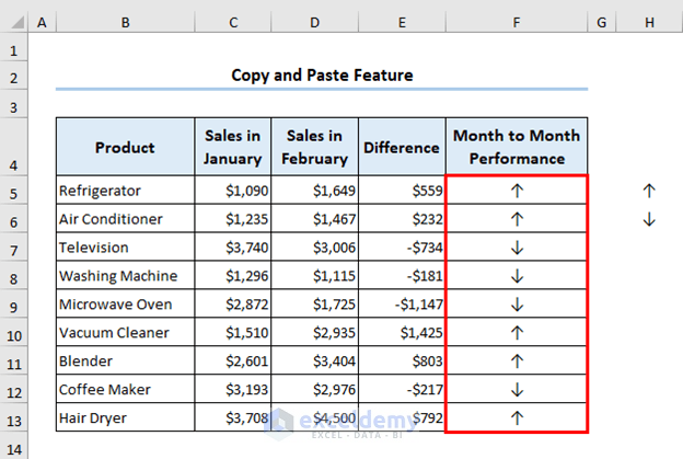
Method 3 – Insert Block Arrows from the Shapes Option
- Go to the Insert tab >> Select Shapes >> Choose an arrow.
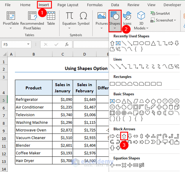
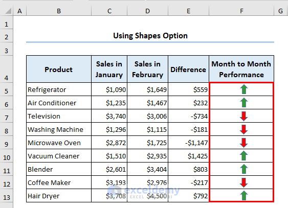
- Excel will insert an arrow. We changed the color from the Fill Color section for better visualization.
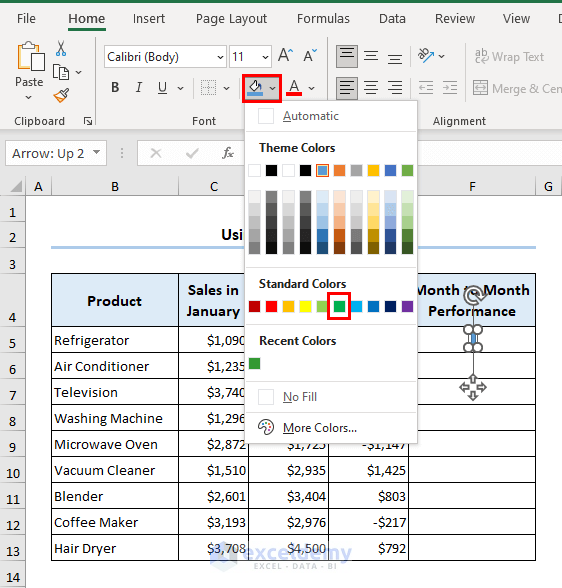
- Insert the rest of the arrows similarly. We set the down arrow to be red.
Method 4 – Use Conditional Formatting to Insert Arrows in Excel
- We have calculated the difference twice and placed the second result in a separate column.
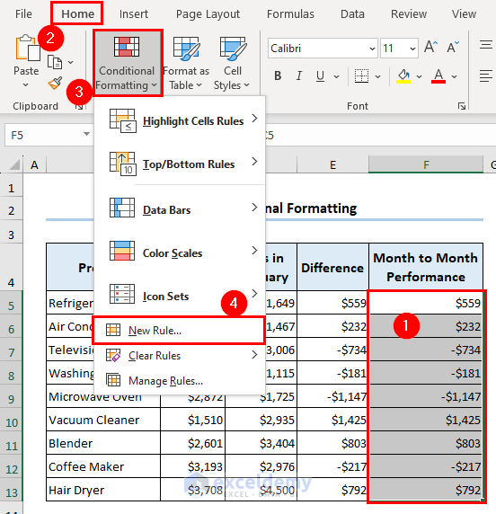
- Select the range F5:F13 >> Go to the Home tab >> Select Conditional Formatting >> Choose New Rule.
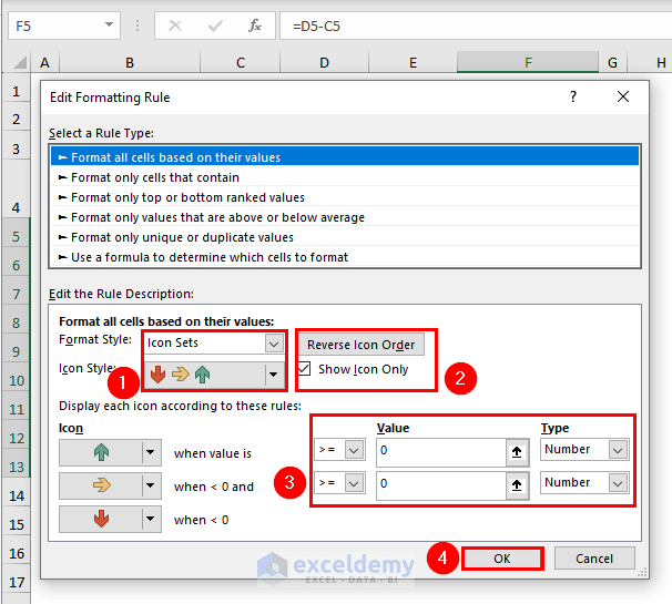
- Choose the Format Style and Icon Style >> check the ‘Show Icon Only’ box >> select the Value and Type >> click OK.
- Excel will insert the arrows.
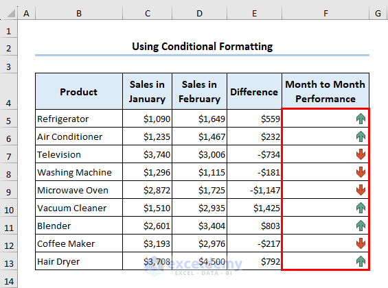
The rule states that Excel will show a green upward arrow when you have a positive number. For a negative number, Excel will show a red downward arrow.
Method 5 – Use Special Fonts to Insert Arrows
- Use the following formula on cell F5 and apply AutoFill to cell F13.
=IF(E5>0,CHAR(233),CHAR(234))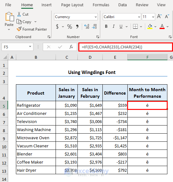
Excel returns some characters. Do not worry about them for now.
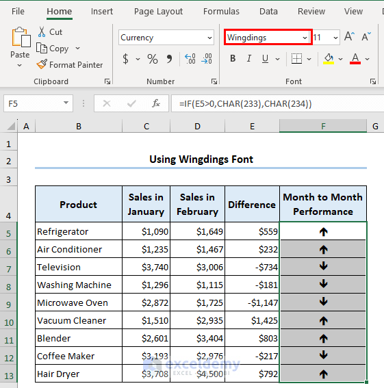
- Change the font to Wingdings to get the arrows.
Method 6 – Insert Arrows Using the Custom Format Option
- Select the range F5:F13 where you want to insert arrows.
- Go to the Home tab >> choose the icon shown at the bottom of the Number group >> select Custom formatting >> then use the following format and press OK.
[Green] $0 ↑;[Red] -$0 ↓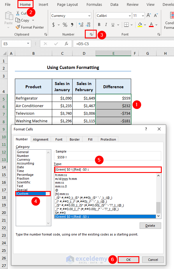
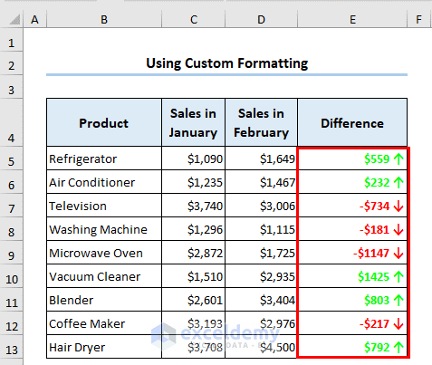
- Excel will do the rest.
How to Insert Arrows in Column Chart
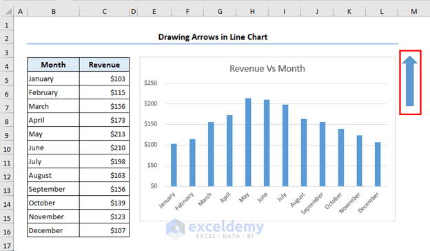
You can insert arrows in a column chart to look sharp and attractive. For example, insert the upward arrow in this column chart.
- We inserted the arrow from the Shape option.
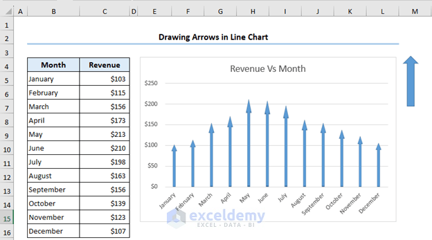
- We copied the shapes and pasted them into the chart’s columns. Excel will change the shape of the columns.
How to Insert Arrows into a Line Chart
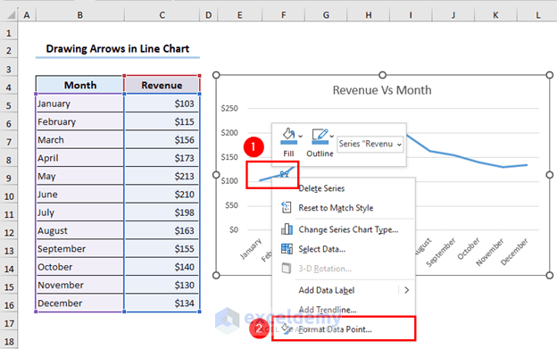
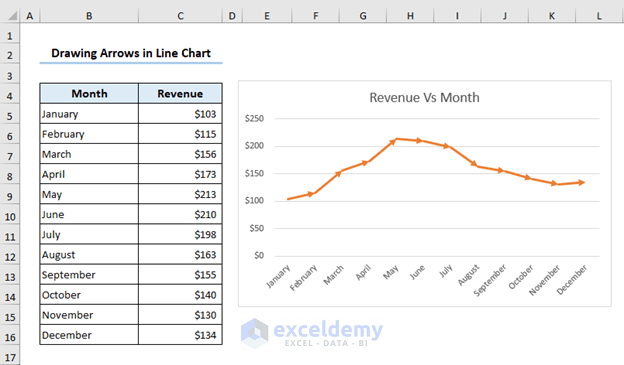
- Select the line to activate only a unit portion >> right-click and select Format Data Point.
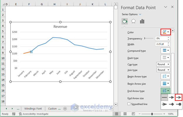
- From the Fill & Line section, change the color of the chart.
- Select the desired arrow from the End Arrow Type section.
- Excel will insert arrows in each unit line.
How to Insert Curved Arrows
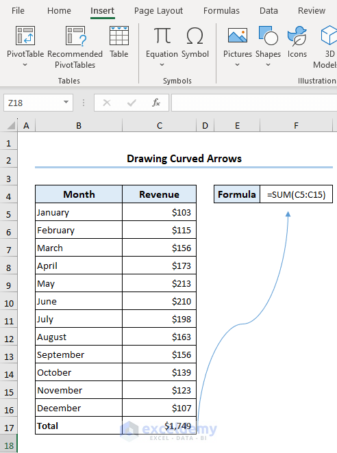
- Insert a curved arrow from the Shapes option.
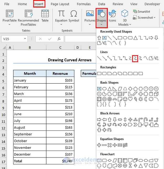
- Place it correctly.
Uses of Arrows in Excel
Arrows in Excel have multiple practical uses:
- Sorting: Sort data in ascending or descending order.
- Conditional Formatting: Use arrows to indicate trends or variances.
- Data Analysis: Trace dependents or precedents to understand cell relationships.
- Navigation: Scroll through cells horizontally or vertically.
- Charting: Add arrows to highlight significant points.
These are some common uses of arrows in Excel.
Things to Remember
- Be careful when positioning the arrows.
- Be consistent with colors, line styles, and thicknesses of arrows.
Frequently Asked Questions
1. Can I customize the appearance of arrows in Excel?
Ans: Yes, you can customize the appearance of arrows by changing their color, line style, thickness, and size. Use the formatting options in the “Format” or “Shape Format” tab to make desired modifications.
2. Can I remove arrows in Excel after inserting them?
Ans: Yes, you can remove arrows in Excel. Simply select the arrow shape you want to delete and press the “Delete” or “Backspace” key, or right-click on the arrow and choose the “Delete” option from the context menu.
3. How can I use arrows for sorting data in Excel?
Ans: To sort data using arrows, click on the arrow icon in the column header of the data you want to sort. Choose “Sort A to Z” or “Sort Z to A” from the drop-down menu to arrange the data in ascending or descending order, respectively.
Arrows in Excel: Knowledge Hub
Download Practice Workbook
Download this workbook and practice.
<< Go Back to Excel Symbols | Learn Excel
Get FREE Advanced Excel Exercises with Solutions!

