Method 1 – Use of ‘Paste Link’ Option to Connect Several Cells from a Different Worksheet
Steps:
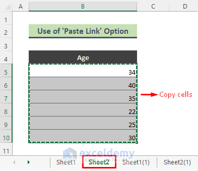
- Go to Sheet2 and copy the range of multiple cells (here B5:B10).
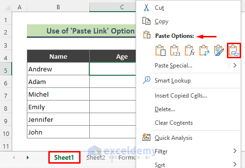
- Go to Sheet1, and put the cursor where you want to paste the data (Here, Cell C5). Right-click on Cell C5 and click on the Paste Link icon from the Paste Options (see screenshots).
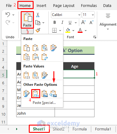
- To get the Paste Link option, follow the following path: Home > Clipboard > Paste > Other Paste Options > Paste Link.
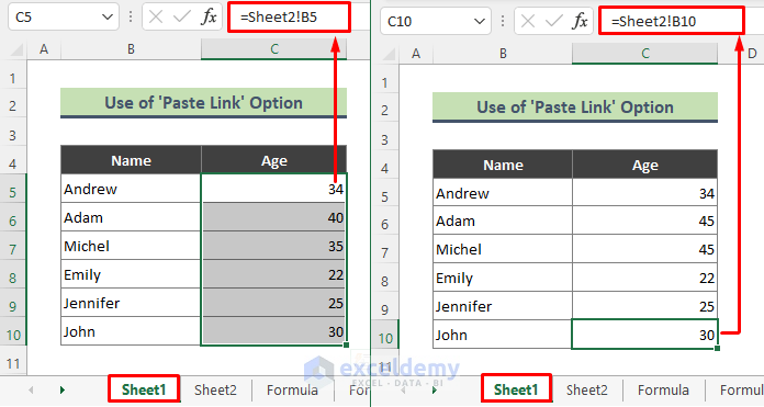
- Get the below output. All the ages from Sheet 2 are now pasted to Sheet1 and these data are connected through links. If you change any of the ages in Sheet2, it will be automatically updated in Sheet1.
Method 2 – Link Multiple Cells from Another Worksheet Using Excel Formula
Steps:
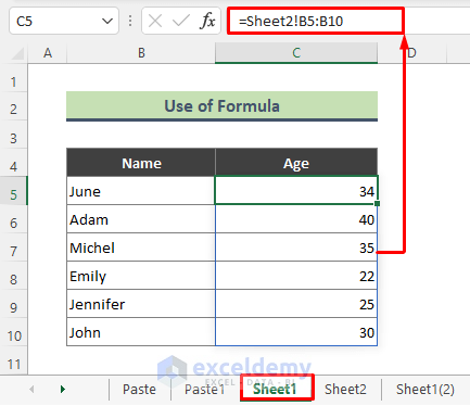
- Type the below formula in Cell C5 and press Enter from the keyboard.
=Sheet2!B5:B10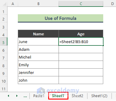
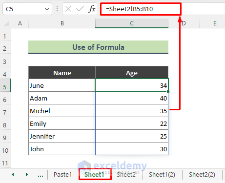
- Excel will return the following output. From the below screenshot, you can see that the above formula returns the result as an array. The result is linked to multiple cells of Sheet2.
⏩ Note:
You can use the above formula manually. To illustrate, follow the steps.
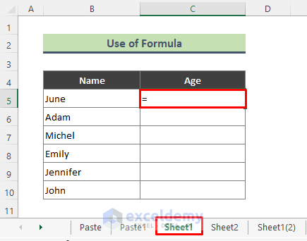
- Type an equal to (=) sign in Cell C5 of Sheet1.
- Go to Sheet 2, select the range of cells to whom you want to put the link and press Enter.
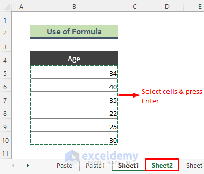
- Pressing Enter in Sheet2, excel will bring you to Sheet1, and thus two sheets are linked as shown in the screenshot below.
Method 3 – Apply Excel Function to Link Several Cells from Another Worksheet
Steps:
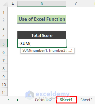
- Go to Sheet1, and type the function as shown in the below screenshot, but do not enter the function’s arguments here.
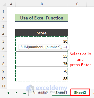
- Go to another sheet (Sheet2), select multiple cells (here, B5:B10), and hit Enter.
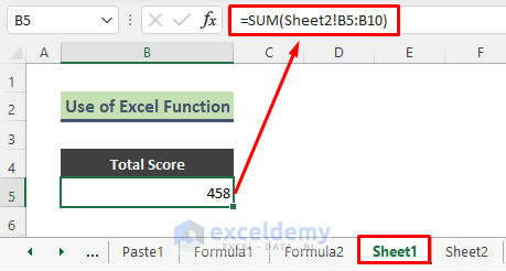
- Excel will direct us to Sheet1 and we get the total scores. If you change any of the scores in Sheet2, the total score will change in Sheet1 accordingly.
Method 4 – Use Plus (+) Sign to Connect Multiple Cells from Other Excel Sheet
Steps:
- Go to Sheet1, type ‘+’ in Cell B5, but do not press Enter.
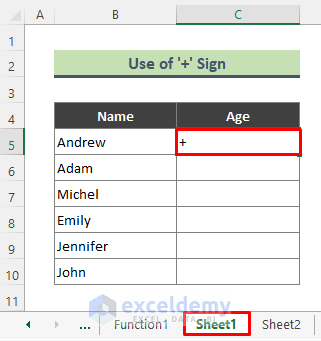
- Go to Sheet2, select the below range of cells, and hit Enter.
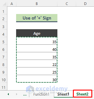
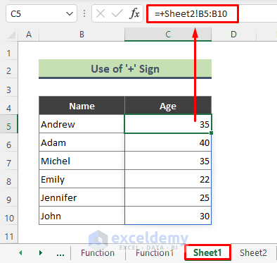
- Excel will take us to Sheet1, and two sheets are linked, as displayed in the screenshot below.
Method 5 – Link Multiple Cells from Different Excel Workbooks
Steps:
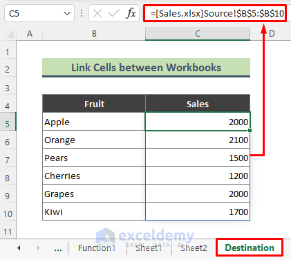
- Go to the workbook that has the worksheet named ‘Destination’ and type the formula below.
=[Sales.xlsx]Destination!$B$5:$B$10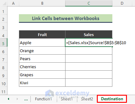
- Press Enter from the keyboard.
- All the sales data of the ‘Source’ worksheet is linked to the ‘Destination’ worksheet. If you change any data in the ‘Source’ worksheet it will dynamically change the data in the ‘Destination’ worksheet too.
Turn On Automatic Calculation While Linking Worksheet in Excel
When you link two excel sheets, changing in source worksheet data updates the destination worksheet data automatically. To ensure the automatic data update, make sure you have turned on the Automatic Calculation Options. Go to Formulas > Calculation Options > Automatic.

Things to Remember
- While linking worksheets, make sure the cell formatting of both the source and destination worksheet should be similar. Otherwise, after linking, data might be displayed differently, which will cause confusion.
- If you link multiple cells between worksheets from different workbooks that are located in different folders, you have to enter the source workbook’s file path in the linking formula.
Download Practice Workbook
You can download the practice workbook that we have used to prepare this article.
Related Articles
- How to Link Cells for Sorting in Excel
- How to Link Tables in Excel
- How to Stop Cell Mirroring in Excel
- How to Keep Formatting in Excel When Referencing Cells
- How to Automatically Link a Cell Color to Another in Excel
- How to Link Cells in Same Excel Worksheet
<< Go Back To Excel Link Cells | Linking in Excel | Learn Excel
Get FREE Advanced Excel Exercises with Solutions!

