Linking Excel Sheets to a Summary Page: 4 Easy Methods

Method 1 – Use Consolidate Command to Link Excel Sheets to a Summary Page

Step 1:

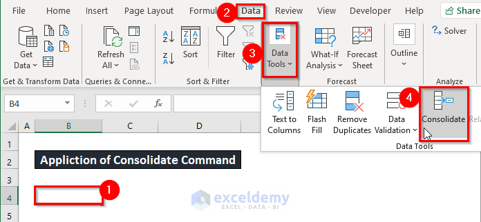
• Select the cell After that, from your Data ribbon, go to,

 Data → Data Tools → Consolidate

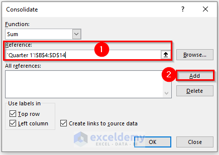
• A  Consolidate dialog box will appear in front of you. From the Consolidate dialog box, type ‘Quarter 1’!$B$4:$D$14 in the Reference press Add option.

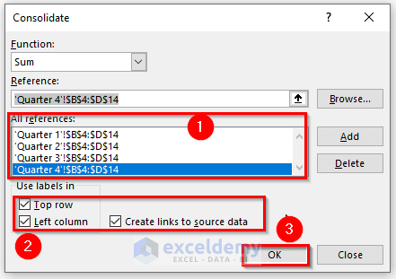
• Add the rest of the sheet value. Check the Top row, Left column, and Create links to source data like the below screenshot. Press OK.

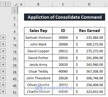
• You will be able to link Excel sheets to a summary page, which has been given in the screenshot below.

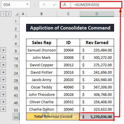
• We will sum up the total revenue earned by the sales representatives using the SUM function like the below screenshot. The return of the SUM function is $5,270,036.00.

Step 2:

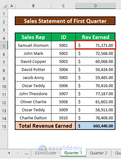
• After linking Excel sheets to a summary page, we will check whether it works or not. Change any value of the source data. We will change the revenue earned by Samuel Jhonson from $51,371.00 to $71,371.00.

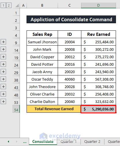
• We will notice that the total revenue earned is changed from $5,270,036.00 to $5,290,036.00 automatically which has been given in the below screenshot.

Method 2 – Perform Hyperlink Command to Link Excel Sheets to a Summary Page

Step 1:

• Select the cell After that, from your Insert ribbon, go to,

 Insert → Links → Link

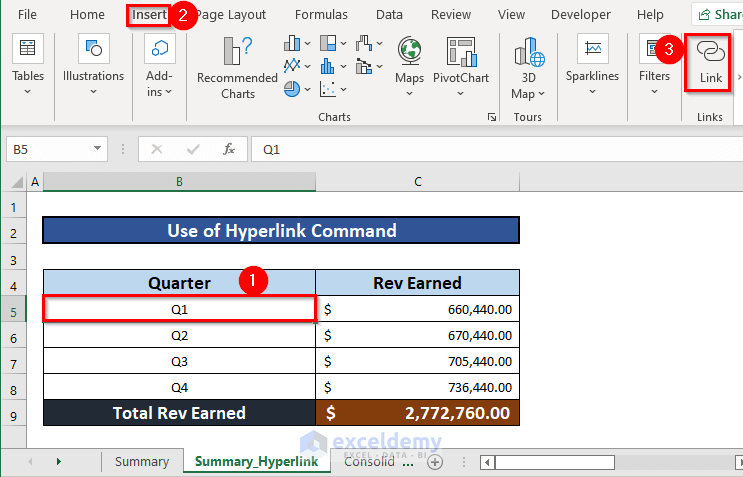
• A Insert Hyperlink dialog box will appear in front of you. From the Insert Hyperlink dialog box, select Place in This Document under the Link to select ‘Quarter 1’ under the or select a place in this document drop-down list. Press OK.

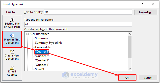
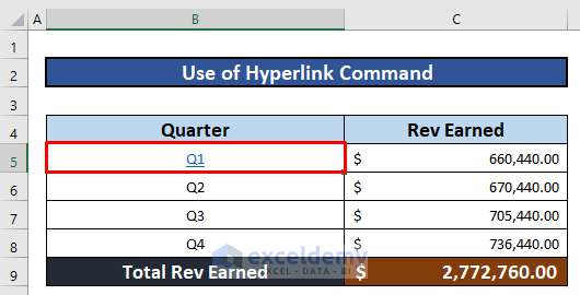
• You will be able to link the ‘Quarter 1’ sheet with the Summary_Hyperlink sheet in cell B5.

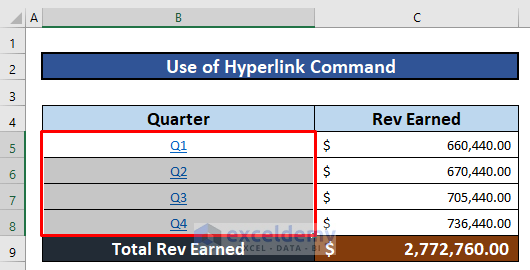
• You can link the rest of the sheets with the Summary_Hyperlink sheet like the screenshot below.

Step 2:

• Click on any of the cells and it will take you to the respected worksheet.

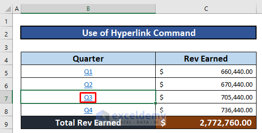
• And our job is done!

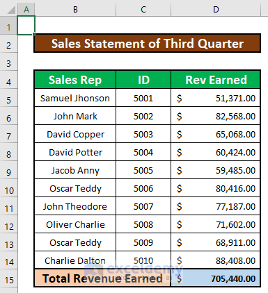
Method 3 – Define Selection Portion to Link Excel Sheets to a Summary Page

Steps:

• Select cells B5 after that, give a name of the selected range, and the name is Group. Press on the left-top box and type that name like the below screenshot.

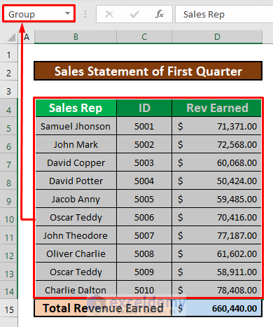
• Select cell B5 and type the below formula. The formula is,

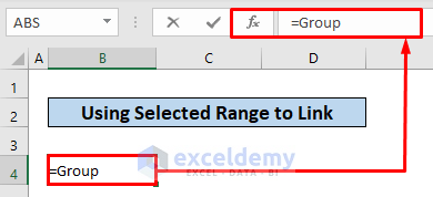
• Simply press ENTER on your keyboard, and you will get the return of that function with linking.

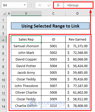
• After linking Excel sheets to a summary page, we will check whether it works. To do that, change any value of the source data. We will change the revenue earned by Samuel Jhonson from $51,371.00 to $61,371.00.

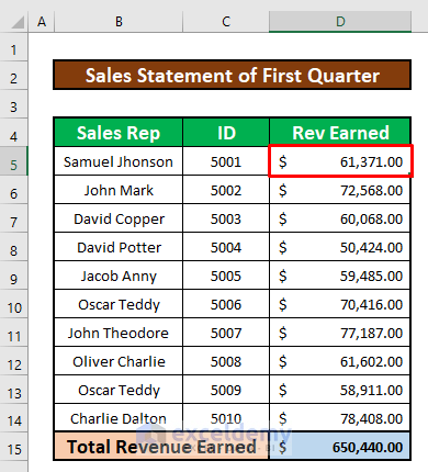
• We will notice that the revenue earned by Samuel Jhonson is changed from $51,371.00 to $61,371.00 automatically which has been given in the below screenshot.

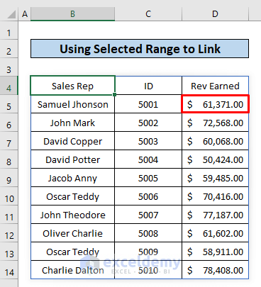
Method 4 – Linking Excel Sheets to a Summary Page Manually

Steps:

• Select cell C5 and type =.

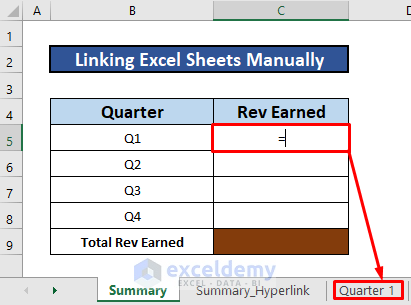
• Go to the ‘Quarter 1’ sheet, and select cell D15.

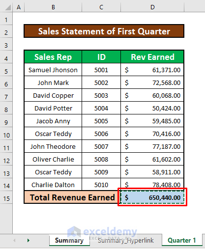
• Press ENTER on your keyboard, and you can link the ‘Quarter 1’ sheet with the sheet named Summary.

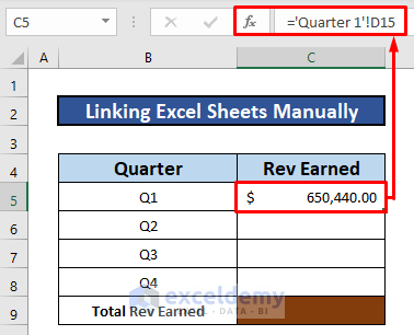
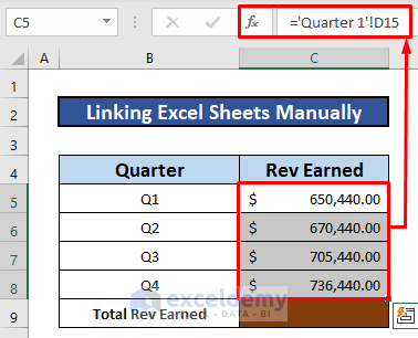
• Linking the sheets ‘Quarter 2’, ‘Quarter 3’, and ‘Quarter 4’ with the sheet named Summary which has been given in the below screenshot.

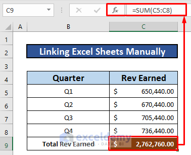
• We will sum up the total revenue earned by the sales representatives using the SUM function like the below screenshot. The return of the SUM function is $2,762,760.00.
• To check whether the linking works, repeat step 2 of method 1.

Things to Remember

➜ While a value can not found in the referenced cell, the #N/A! error happens in Excel.

➜ #DIV/0! error happens when a value is divided by zero(0) or the cell reference is blank.

Download Practice Workbook

Download this practice workbook to exercise while you are reading this article.

Related Articles

• How to Automatically Update One Worksheet from Another Sheet in Excel
• Transfer Data from One Excel Worksheet to Another Automatically
• How to Reference Cell in Another Excel Sheet Based on Cell Value
• How to Make Excel Look Like an Application
• Transfer Specific Data from One Worksheet to Another for Reports

<< Go Back To Excel Link Sheets | Linking in Excel | Learn Excel