How to Lock Columns in Excel (4 Methods)

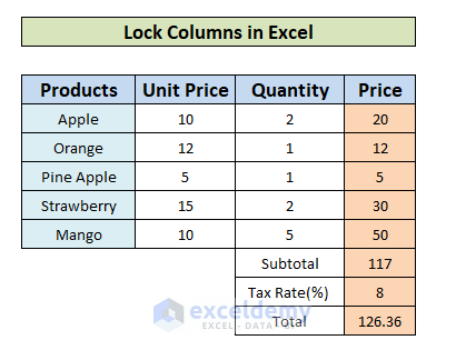
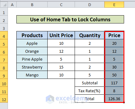
The dataset below will be used for illustration.

By default, an Excel worksheet has all its cells locked. But, it has no effect until the sheet is protected. To check this:

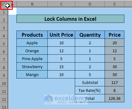
• Click the Select All button at the top-left corner of the spreadsheet.

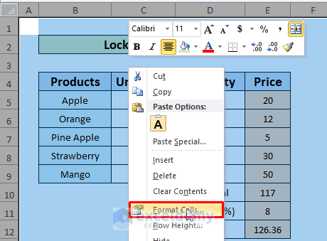
• Right-click to open up the context menu and choose the Format Cells.

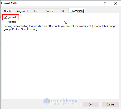
• In the Format Cells window, the Protection tab shows the Locked Checkbox selected by default.

Method 1 – Lock All Columns with Protect Sheet in Excel

• In the Excel Ribbon, navigate to the Review tab and select Protect Sheet.

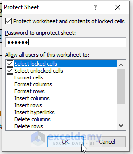
• Protect with Password: In the Protect Sheet window put a suitable password that will be required to unprotect the sheet.

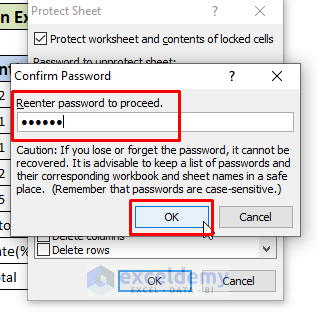
• Another window will pop up to confirm the password. Put the same password from the previous step and hit OK.

• Click on any cell on the spreadsheet, it will show a warning.

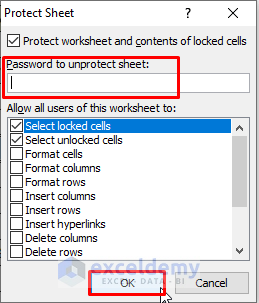
• Protect without Password: Leave the password input box and just click OK.

Method 2 – Lock Specific Columns from the Home Tab 

• Click the upper-left button to select the whole worksheet.

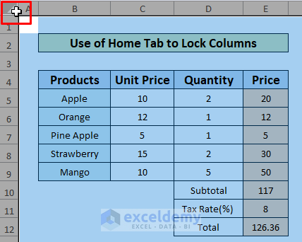
• In the Home Tab, click the arrow from the Alignment.

Another Way: From the Home Tab click the Orientation and choose Format Cells Alignment from the dropdown.

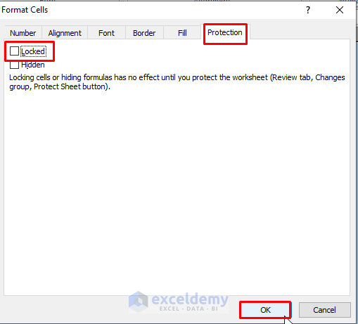
• In the Format Cells window, uncheck the Locked checkbox from the Protection Tab and hit OK.

• Select the Price column.

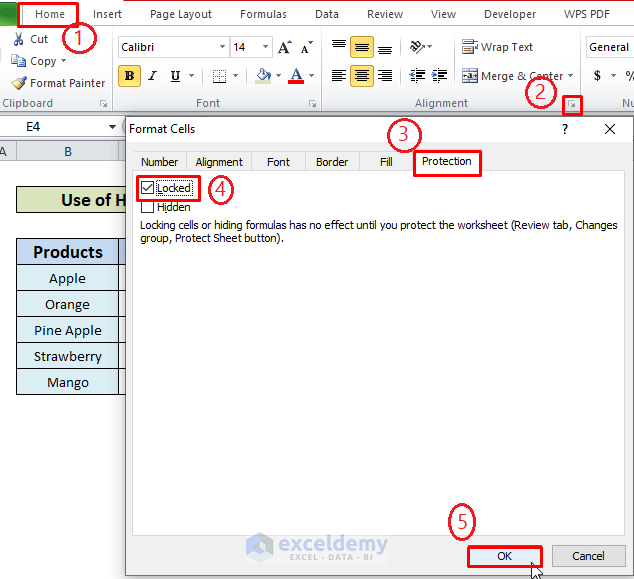
• In the Home Tab, click the arrow from the Alignment.
• In the Format Cells window, check the Locked checkbox from the Protection Tab and hit OK. It’ll lock the selected Price column.

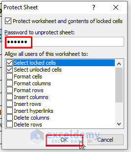
• Protect with Password: In the Protect Sheet window put a suitable password that will be required to unprotect the sheet. You can also select different options to allow user actions to the worksheet by checking the square boxes.

• A window will pop up to confirm the password. Put the same password from the previous step and hit OK.

• When any cell is clicked on the Price column, it will show a warning.

• Protect without Password: Leave the password input box and click OK.

• If any value in the Unit Price or Quantity column is changed, it will make adjustments in the Price column accordingly.

Method 3 – Using the Context Menu to Lock Selected Columns in Excel

• Click the upper-left button to select the whole worksheet. Use right-click to select the Format Cells

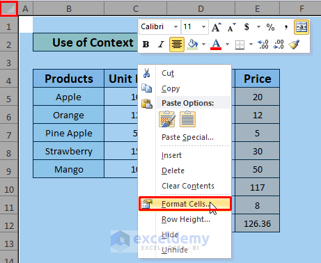
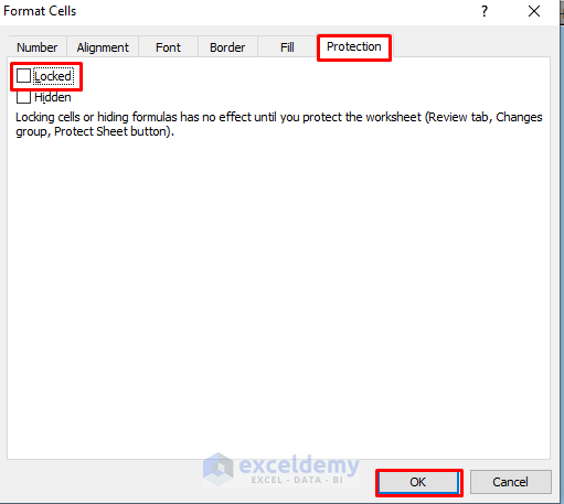
• In the Format Cells window, uncheck the Locked checkbox from the Protection Tab and hit OK. This unlocks the whole worksheet.

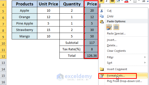
• Select the Price column of the dataset and right-click to select the Format Cells option.

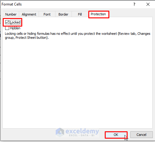
• To lock the selected column, check the Locked checkbox from the Protection Tab and click OK.

• Choose the Protect Sheet option of the Review Tab.

To complete the process, follow either of the two steps described in the previous method:

• Protect with Password
• Protect without Password

Method 4 – Find and Lock the Formula Columns

• Unlock the worksheet.
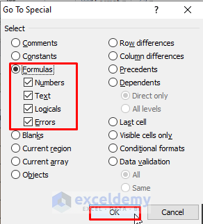
• Go to the Home tab, choose Find & Select, and click on Go to Special.

• From the Go to Special window select Formulas options and click OK.

• All the cells with formulas are selected (the Price column in our example).

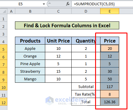
• To make the column locked, follow Method 2.

Download the Practice Book 

Related Articles

• How to Swap Columns in Excel
• How to Autofit All Columns in Excel

<< Go Back to Learn Excel