Method 1 – Using the VLOOKUP Function to Lookup a Partial Text Match in Excel
In the following picture, there is a table containing the marks in different subjects for some students in an exam. Based on the partial match of a text from Column B, we’ll extract the marks in a subject for a student. Let’s look for the text “Tick” in the column of Name. We’ll find out the actual name of that student and then extract the marks in math of the corresponding student from the table.
The generic formula of this VLOOKUP function is:
=VLOOKUP(lookup_value, table_array, col_index_number, [range_lookup])
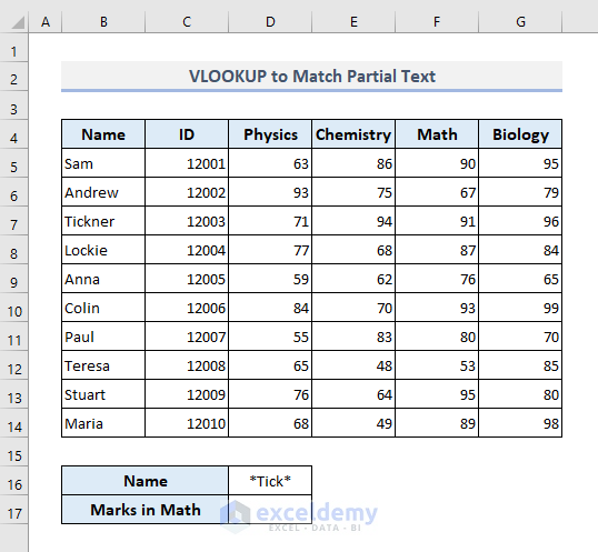
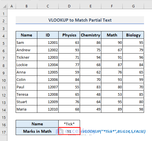
- Since we’re going to pull out the marks in math of a student whose name contains the text “Tick”, the required formula in the output cell D17 will be:
=VLOOKUP(D16,B5:G14,5,FALSE)Or,
=VLOOKUP("*Tick*",B5:G14,5,FALSE)- After pressing Enter, you’ll see the marks in math for Tickner.
Method 2 – Combining Excel INDEX-MATCH Functions to Lookup a Partial Text Match
We’ll use the same dataset.
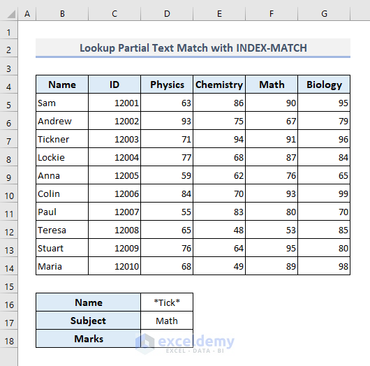
- The required formula in the output cell D18 will be:
=INDEX(B5:G14,MATCH(D17,B5:B14,0),MATCH(D17,B4:G4,0))Or,
=INDEX(B5:G14,MATCH("*Tick*",B5:B14,0),MATCH(D17,B4:G4,0))- Press Enter and the formula will return “91”- the marks Tickner has obtained in math.
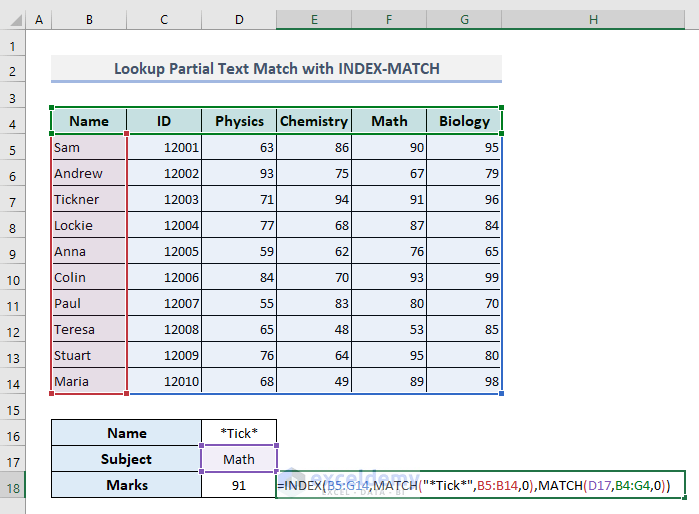
In this formula, the two MATCH functions define the row and column numbers of the student’s name and the subject, respectively. INDEX function then returns the value at the intersection of those defined row and column numbers from the array.
Method 3 – Applying Excel XLOOKUP to Lookup a Partial Text Match with a Wildcard Character
The XLOOKUP function searches a range or an array for a match and returns the corresponding item from a second range or array. The generic formula of this function is:
=XLOOKUP(lookup_value, lookup_array, return_array, [if_not_found], [match_mode], [search_mode])
Now we’ll use this XLOOKUP function directly to extract the marks in math of the student whose name contains the text “Tick” inside.
- In the output cell D18, the required formula will be:
=XLOOKUP("*"&D16&"*",B5:B14,F5:F14,,2)- After pressing Enter, you’ll find a similar output as found in the previous two examples.
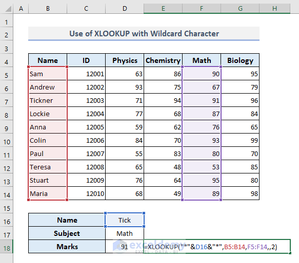
In this function, we’ve used “2” as the [match_mode] argument that denotes the wildcard character match. If you don’t use this argument, the function will return #N/A error, since the function will look for the exact match instead of the wildcard character match.
Method 4 – Joining XLOOKUP, ISNUMBER, and SEARCH Functions to Lookup a Partial Text Match
- The required formula in the output cell D18 will be:
=XLOOKUP(TRUE,ISNUMBER(SEARCH(D16,B5:B14)),F5:F14)- Press Enter.
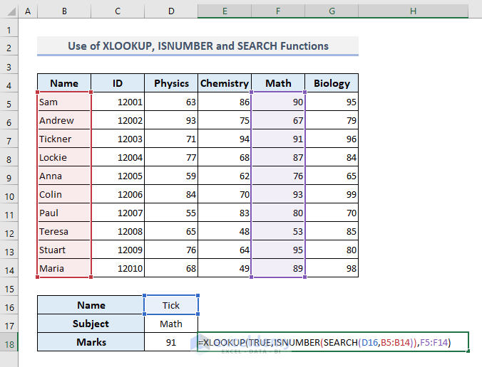
How Does the Formula Work?
- The SEARCH function looks for the text ‘Tick’ in the range of cell B5:B14 and returns an array of:
{#VALUE!;#VALUE!;1;#VALUE!;#VALUE!;#VALUE!;#VALUE!;#VALUE!;#VALUE!;#VALUE!}
- The ISNUMBER function then searches for the numeric value in that array and returns another array of boolean values:
{FALSE;FALSE;TRUE;FALSE;FALSE;FALSE;FALSE;FALSE;FALSE;FALSE}
- The XLOOKUP function then looks for the specified boolean value- TRUE in the array found in the previous step and extracts the row number of that value in the array of B5:B14.
- Finally, based on the return array of F5:F14, the XLOOKUP function draws out the marks in math of the student whose name contains the text- ‘Tick’ inside.
Method 5 – Merging Excel FILTER, ISNUMBER, and SEARCH Functions to Lookup a Partial Text Match
- Insert the following formula in the result cell:
=FILTER(F5:F14,ISNUMBER(SEARCH(D16,B5:B14)))- Press Enter.
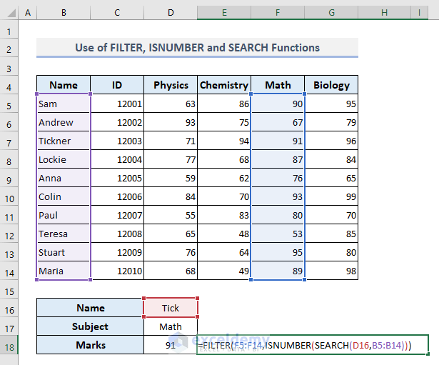
FILTER is available in Excel 365 and Excel 2021 and newer versions.
Download the Practice Workbook
<< Go Back to Partial Match Excel | Formula List | Learn Excel
Get FREE Advanced Excel Exercises with Solutions!

