How to Make a Ledger in Excel (with Easy Steps)

Need to learn how to make a ledger in Excel? If you are looking for such unique tricks, you’ve come to the right place. Here, we will take you through 5 easy and convenient steps in making a ledger in Excel.

What Is a Ledger?

A ledger is an essential document for any organization. It shows us the details of debit and credit and the current balance of that company after every transaction.
Ledger books are usually three types:

Sales Ledger
A sales ledger is a record of the sale of goods or services to customers that are kept by the company. As a result of this ledger, we are able to get the idea of sales profit and income statement.

Purchase Ledger
The Purchase Ledger records the transactions of that company when purchasing goods, services, or products from other organizations. It provides us with visible information on how much the organization paid to other companies.

General Ledger
General Ledger is usually two types:
Nominal Ledger: The nominal ledger provides us with information on earnings, expenses, insurance, depreciation, etc.
Private Ledger: The private ledger keeps track of private information such as salaries, wages, capital, etc. A private ledger is usually not reachable to every person.

Make a Ledger in Excel: Step-by-Step Guidelines

To demonstrate the procedure, we will show you the making approach of a three-month ledger book with the summary in Excel. The procedure is discussed below step-by-step:

Step-01: Create Layout of Ledger in Excel

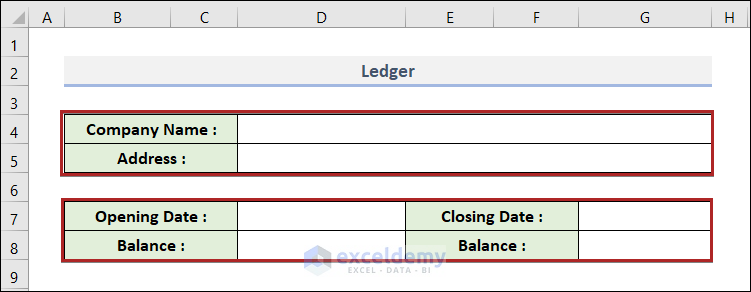
In the first step, we shall construct a space where we can include all the pertinent details about the organization. In this section, we’ll make the appropriate space in each monthly ledger.

First of all, in the range of cells B4:B5, B7:B8, and E7:E8, write down the following entities and format the corresponding cells as the input cells of these values.

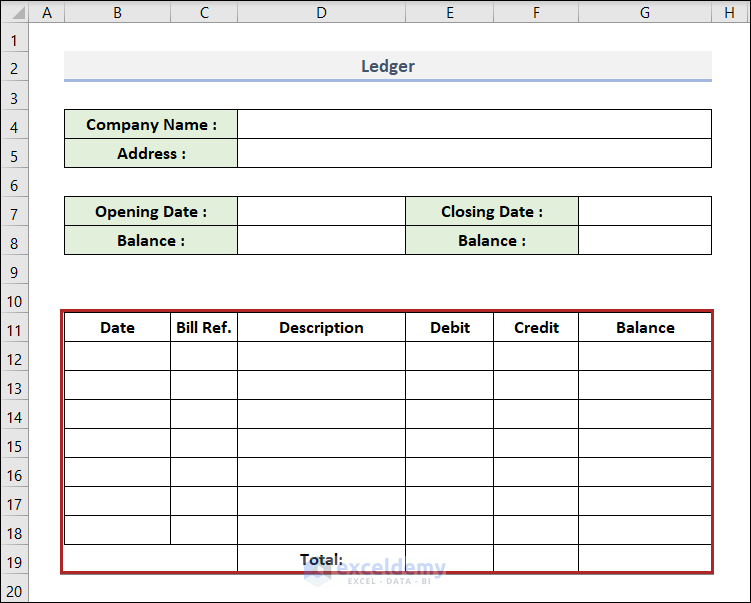
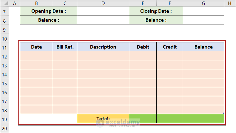
Then, in the range of cells B11:G19, create a tabular format with the following heading titles.
After that, format the cells with the All Border option from the Font group located in the Home tab.

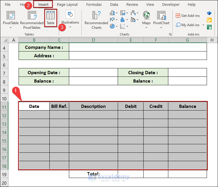
Thirdly, select cells in the B11:G18 range.
Next, go to the Insert tab.
Later, select the Table option from the Tables group.

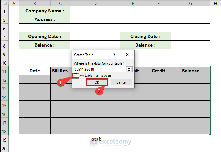
Suddenly, the Create Table input box will open.
Don’t forget to check the box My table has headers.
Then, click on the OK button.

At this moment, we converted the data range into a table.
Now, move to the Table Design tab.
Then, select the Table Style Options group.
After that, uncheck the Filter Button option.

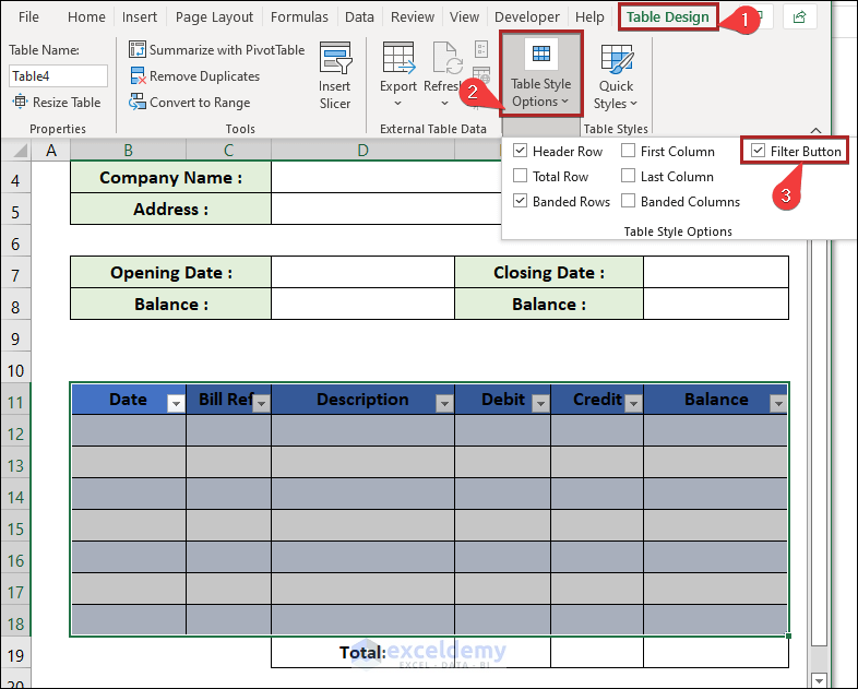
At this moment, the table will show itself without the filtering option.

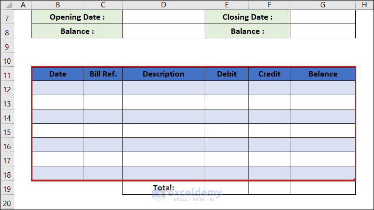
Note: Also, we can do the same work by pressing CTRL+SHIFT+L.

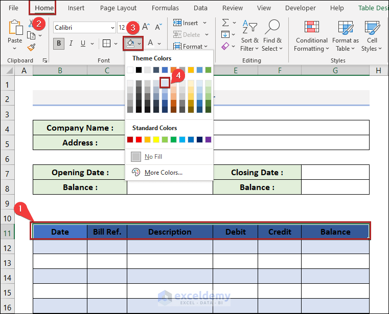
Afterward, select cells in the B11:G11 range.
Now, move to the Home tab.
Next, select the Fill Color drop-down on the Font group.
Later, choose any color according to your preference (here we have chosen Blue, Accent 1, Lighter 80%).

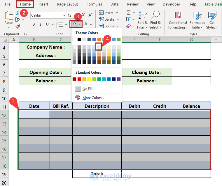
Also, do the same thing to cells in the B12:G18 range with another color (here, we’ve chosen Orange, Accent 1, Lighter 80%).

Thus, the cells in the B11:G19 range look as in the image below.

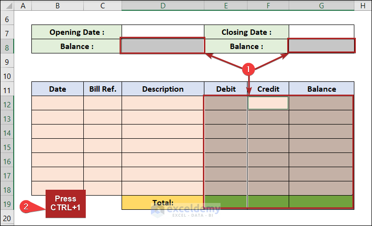
Now, select cells D8, G8, and cells in the range of E12:G19.
After that, press the CTRL key followed by the 1 key on your keyboard.

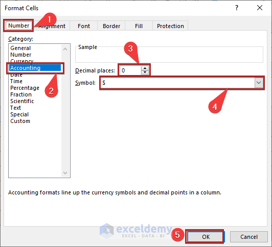
Instantly, the Format Cells dialog box will open up.
Then, go to the Number tab.
Next, select Accounting from the Category.
Later, write down 0 in the box of Decimal places and choose the dollar sign ($) from the Symbol drop-down list.
Lastly, click OK.

Step-02: Make a Monthly Ledger in Excel

In this step, we are going to generate the monthly ledger account dataset to keep the records of our financial activities.

At first, select cell G3 and write down the following formula.

=MID(CELL("filename",A1),FIND("]",CELL("filename",A1))+1,255)&" "&2022

Formula Breakdown
This formula returns the sheet name in the selected cell.

CELL(“filename”, A1): The CELL function gets the complete name of the worksheet
FIND(“]”, CELL(“filename”, A1)) +1: The FIND function will give you the position of ] and we’ve added 1 because we require the position of the first character in the name of the sheet.
255: Excel’s maximum word count for the sheet name.
MID(CELL(“filename”,A1),FIND(“]”,CELL(“filename”,A1))+1,255): The MID function uses the text’s position from start to end to extract a specific substring

Then, press ENTER.

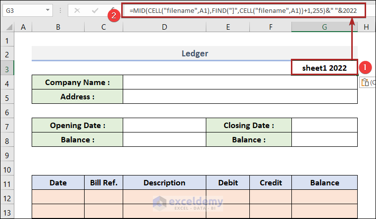
At this point, we can see the name of our Sheet on this cell with 2022.

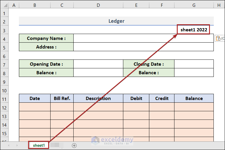
Note: While typing this formula, make sure to enter any cell references on this sheet. Otherwise, the formula won’t work properly. For example, here we’ve entered the reference of cell A1.

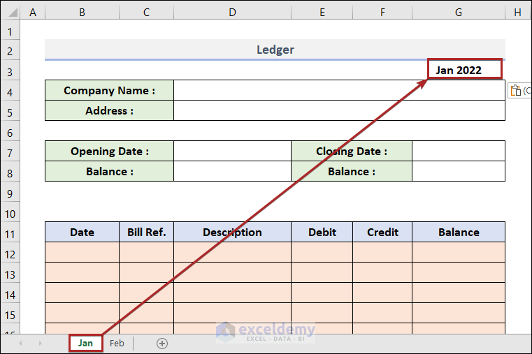
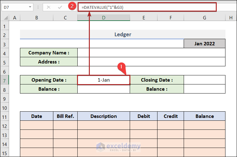
After that, change the name of the sheet to Jan. As we wanna make the ledger for the month of Jan’22. We can easily see that the month’s name is automatically input into cell G3 after changing the name of the sheet.

Then, select cell D7 and put down the following formula.

=DATEVALUE("1"&G3)

The DATEVALUE function converts a date in the form of text to a number that represents the date in Microsoft Excel date-time code.

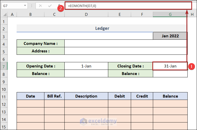
Also, we need the end date of this month.
So, select cell G7 and paste the formula below.

=EOMONTH(D7,0)

The EOMONTH function gives the inferred number of months before or after the start_date. It is the sequential number for the closing day of the month.

At this moment, the worksheet is ready to use as a monthly ledger sheet.

Step-03: Give Some Sample Data as Input into Ledger in Excel

In this third step, we will input sample data into our ledger book. Let’s follow the steps carefully.

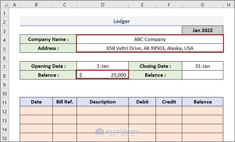
First of all, input the name of the company and address into cells D4 and D5.
Then, put the Balance at the start date in cell D8.

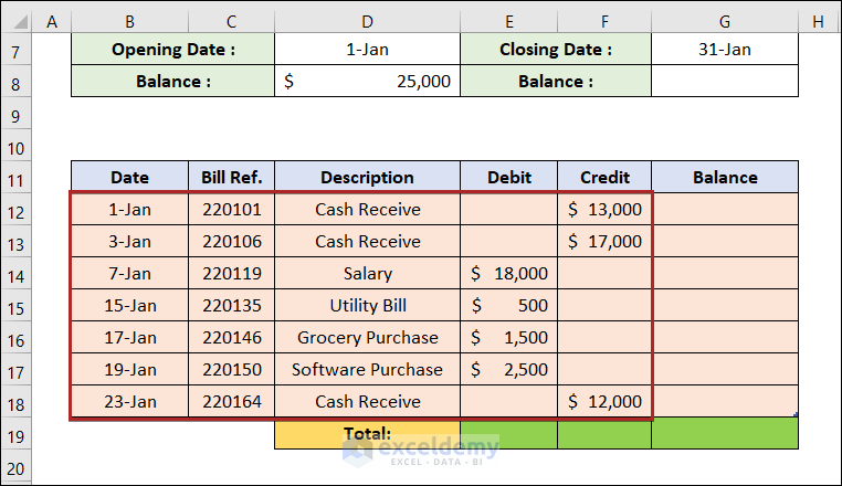
Afterward, fill up the cells in the B12:F18 range with proper data of Date, Bill Ref, Description, Debit, Credit, and Balance.

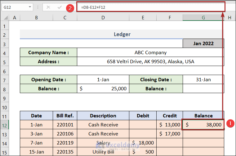
Now, select cell G12 and write down the following formula.

=D8-E12+F12

Here, D8, E12, and F12 represent the Opening Date Balance, Debit, and Credit respectively.

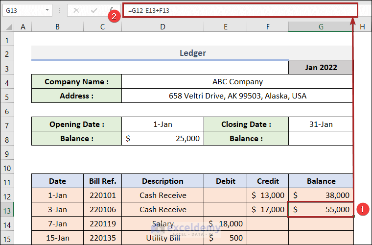
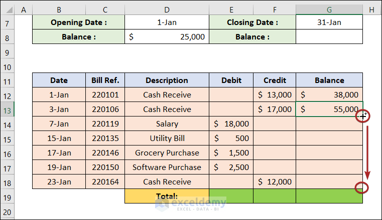
Then, select cell G13 and put down the formula below.

=G12-E13+F13

Here G12, E13, and F13 serve as the corresponding Balance of the previous entries, Debit and Credit.

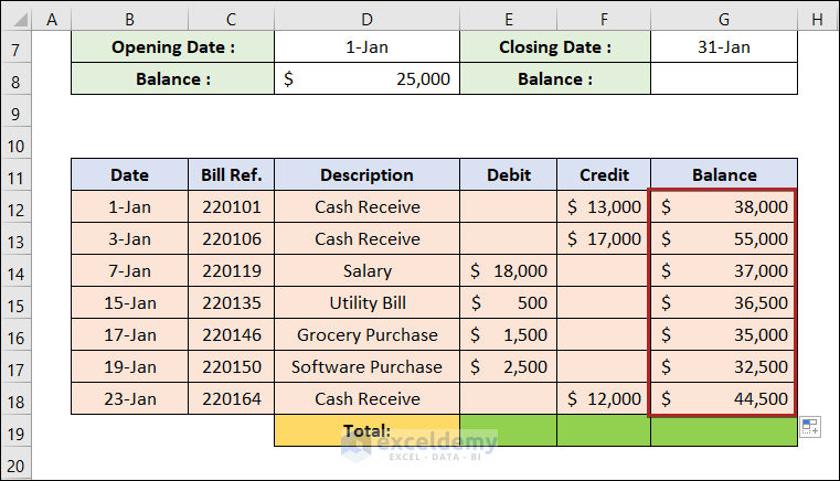
Now, drag down the Fill Handle icon to copy the formula up to cell G18.

In this instance, the Balance column looks like the one below.

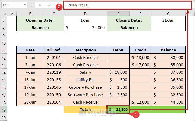
At this point, select cell E19 and write down the following formula.

=SUM(E12:E18)

It calculates the total Debit in the E12:E18 range.

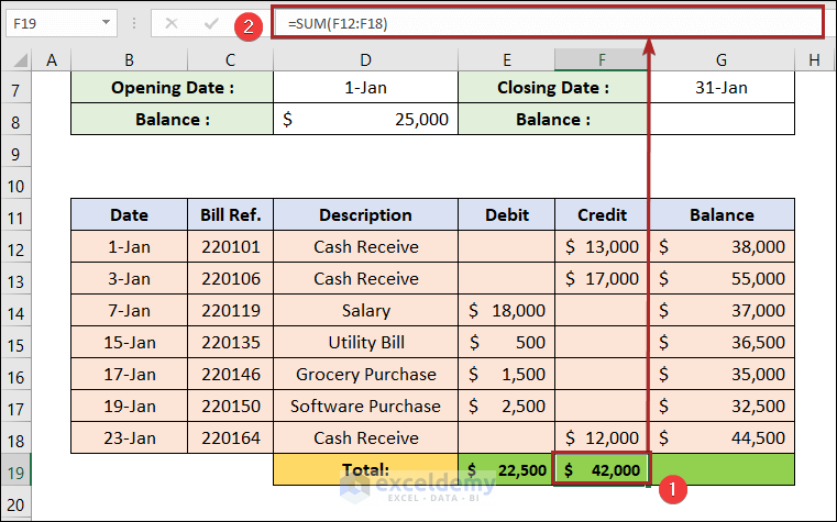
Similarly, select cell F19 and put down the following formula below.

=SUM(F12:F18)

It calculates the total Credit in the F12:F18 range.

Then, select cell G19 and write down the following formula.

=D8-E19+F19

Here, D8, E19, and F19 represent the Opening Balance, Total Debit, and Total Credit consecutively.

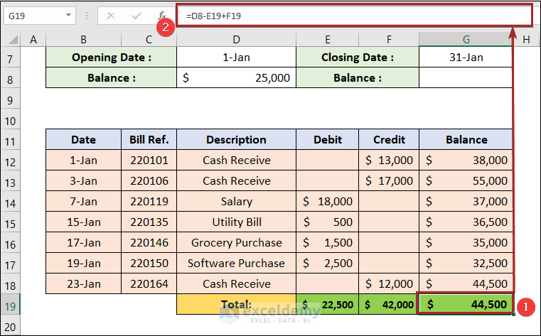
Notice that the amount in cell G18 and in cell G19 are the same. So we can be sure that the calculation is correct. It’s one kind of cross-checking.

Afterward, select cell G8 and put the formula below.

=G19

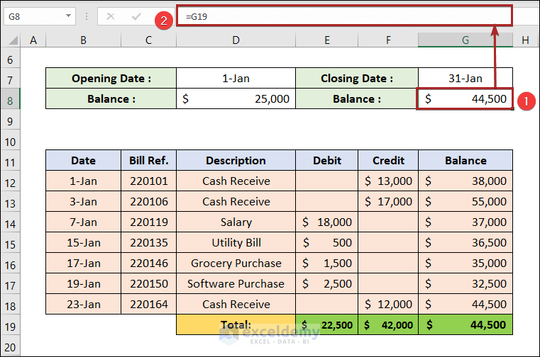
Finally, the ledger for the month of January looks like the image below.

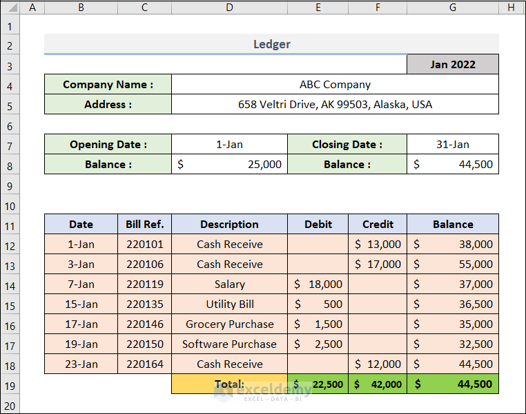
Step-04: Add Other Months

In this step, we’ll create ledgers for other months also. So, let’s just follow these steps.

At the very beginning, right-click on the sheet name Jan.
Then, select Move or Copy from the context menu.

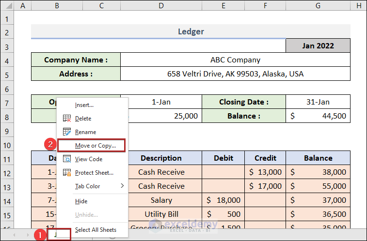
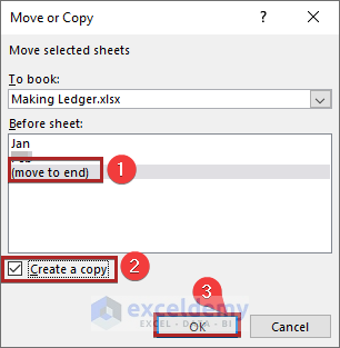
Suddenly, it will open up the Move or Copy dialog box.
Then, select move to end in the Before sheet box.
Obviously, make sure to tick the box of Create a copy.
Finally, click OK.

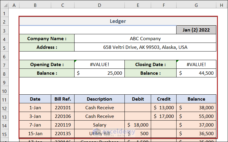
Hence, we created a new sheet Jan (2) by our previous action.

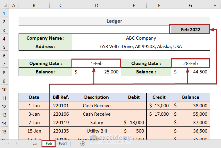
Now, edit the sheet name and make it Feb.
Automatically, the month, Opening Date, and Closing Date will be changed.

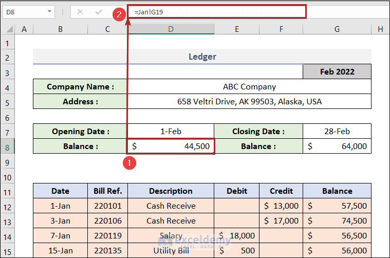
Afterward, select cell D8 and write down the formula below.

=Jan!G19

Here, the Opening Balance is equal to the Closing Balance for January month.

Then, clear the previously entered data for the month of January in the B12:F18 range.

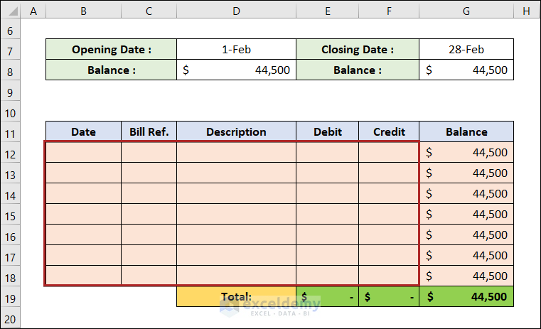
Now, enter the data for the month of February.

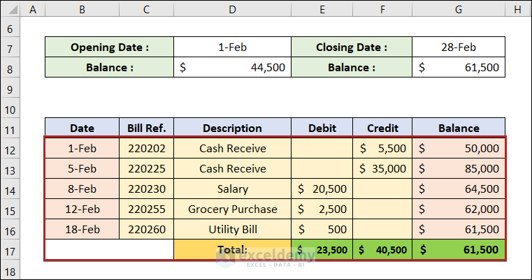
Here, we have entry till Row 16. If we want to add other entries below, we can do that easily. Because we’ve transformed the data range into a table previously.

Firstly, select cell G16.
Then, press the TAB key.

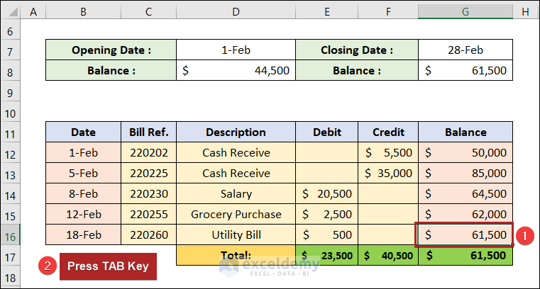
Instantly, it will add another formatted row to input another dataset.

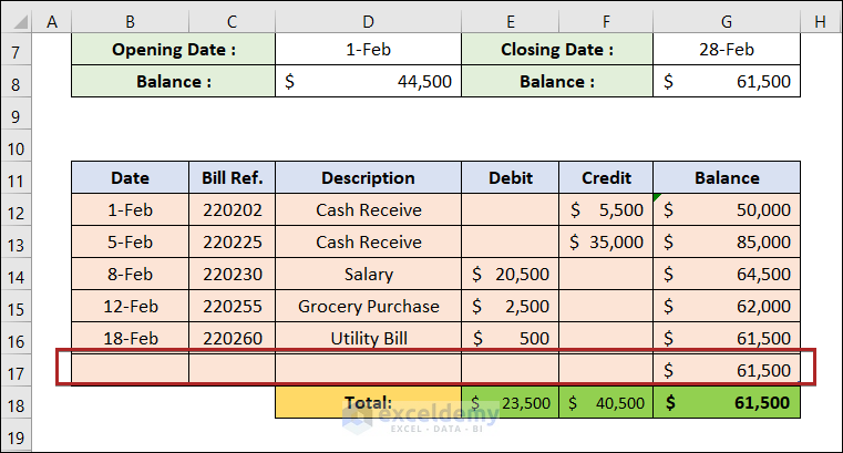
Later, make another entry in this newly created row.

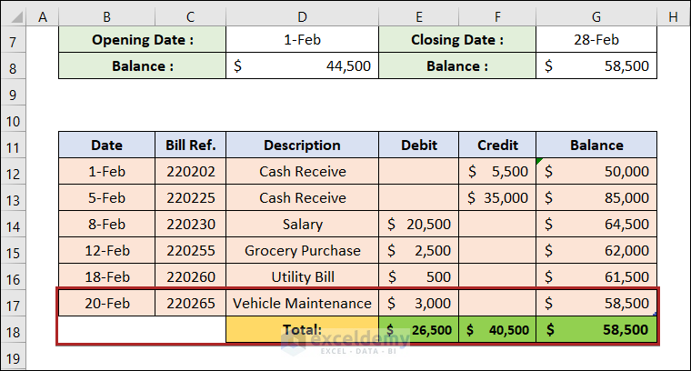
Notice that the Totals in Row 18 and Balance in cell G17 are automatically calculated.

Similarly, follow the previous steps and make the ledger for the month of March.

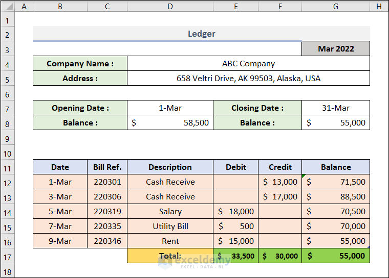
Step-05: Generate a Summary

In the final step, we’ll create a summary of the monthly ledger sheets. Just follow along.

Initially, make the layout just as in the image below.

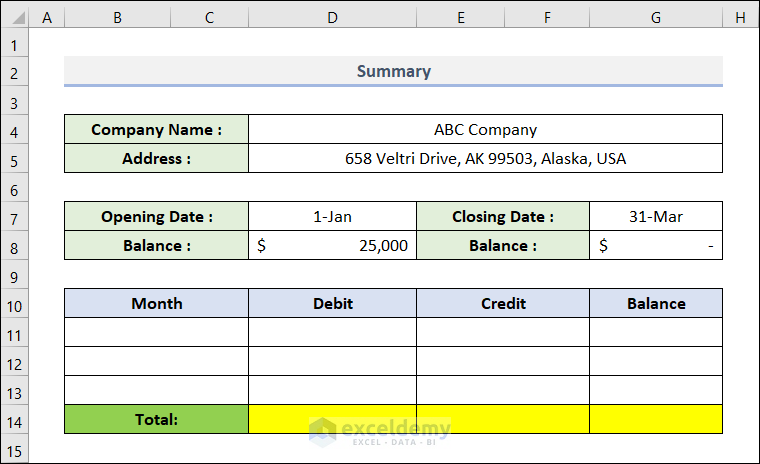
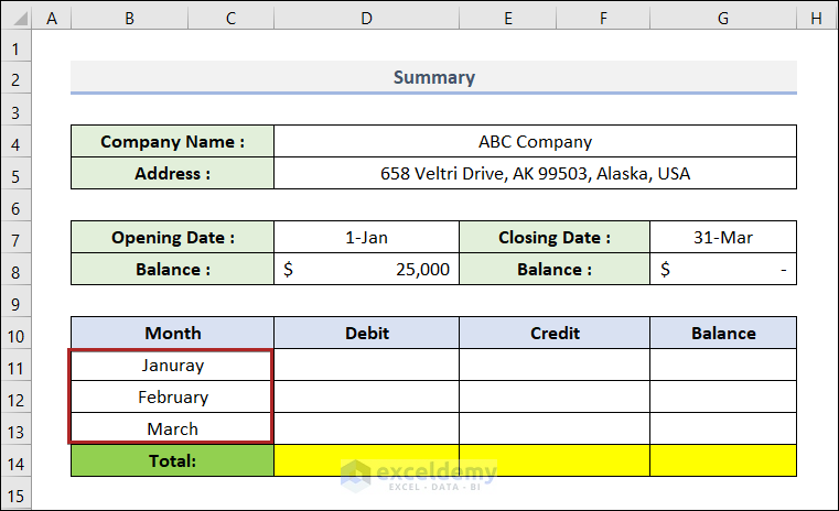
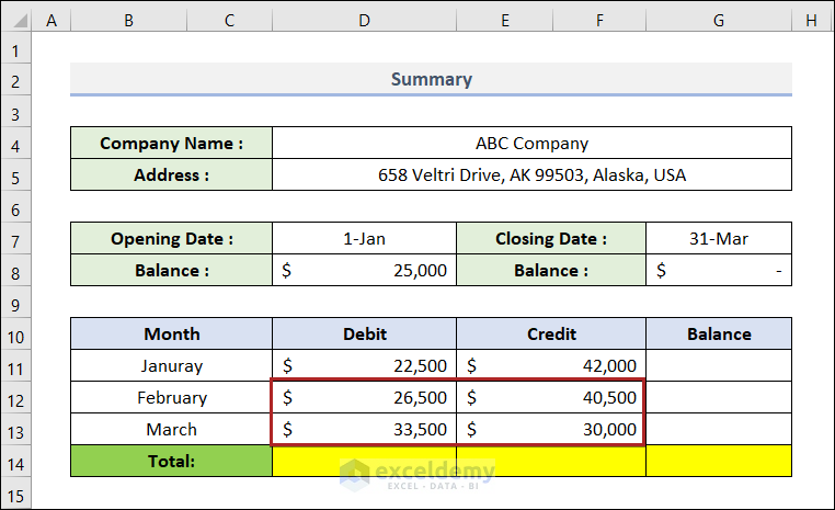
Then, enter the name of the months. Here we’ve made ledgers for the first three months. So, we’re putting these into the cells in the B11:B13 range.

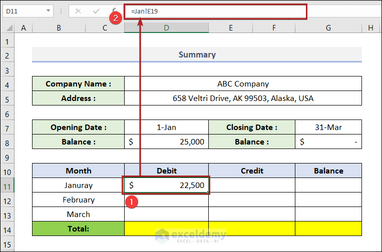
Afterward, select cell D11 and paste the formula below.

=Jan!G19

Here, we’re sourcing this data from cell G19 of the sheet Jan. It contains the Total Debit amount for the month of January.

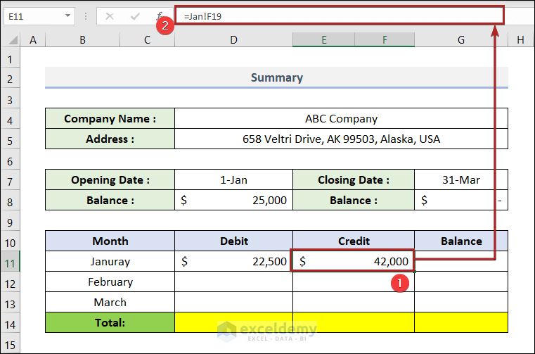
Similarly, get the Total Credit amount for January month in cell F11 using the formula below.

=Jan!F19

Furthermore, get the same values for the month of February and March.

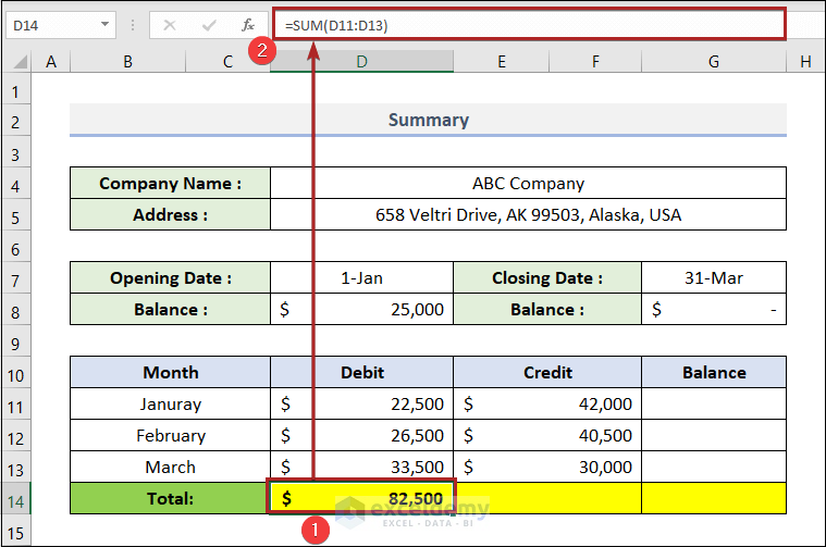
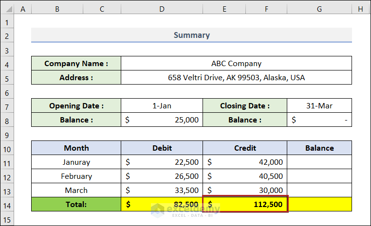
After that, select cell D14 and paste the following formula.

=SUM(D11:D13)

It calculates the Total Debit in these three months.

Also, calculate the Total Credit in cell F14.

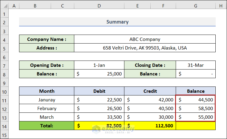
Later, get the Balances from the Ending Balance of each month.

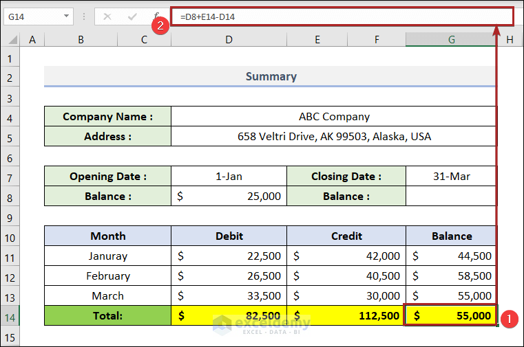
For cross-checking, select cell G14 and write down the following formula.

=D8+E14-D14

Here, D8, E14, and D14 represent the Opening Balance, Total Debit, and Total Credit consecutively.

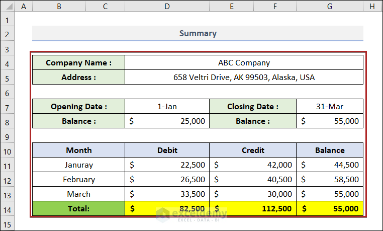
Finally, the Summary looks like the image below.

Read More: How to Make a Bank Ledger in Excel

Download Practice Workbook

You may download the following Excel workbook for better understanding and practice yourself.

Making Ledger.xlsx

Conclusion

This article provides easy and brief solutions to make a ledger in Excel. Don’t forget to download the Practice file. Thank you for reading this article, we hope this was helpful. Please let us know in the comment section if you have any queries or suggestions.

<< Go Back to Ledger in Excel | Excel for Accounting | Learn Excel

Get FREE Advanced Excel Exercises with Solutions!