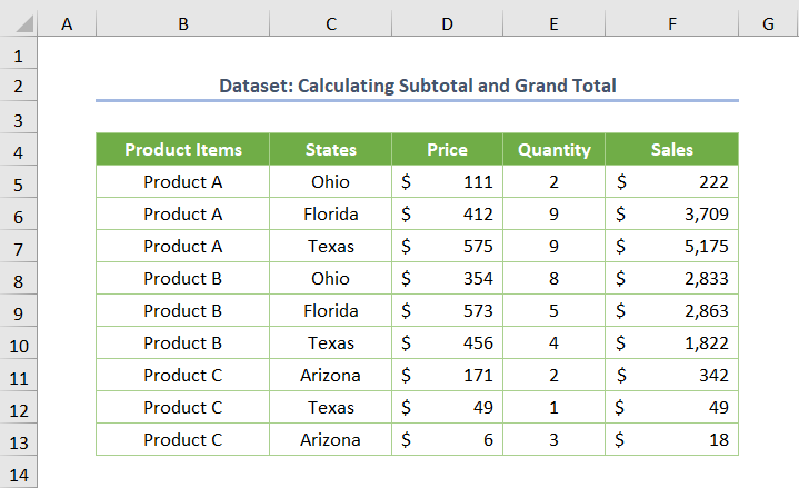
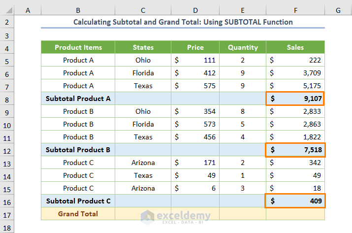
How to Make Subtotal and Grand Total in Excel (4 Methods)

Consider the dataset as shown in the following screenshot. Here, the sales report contains Product Items, States, Price, Quantity, and Sales. We’ll calculate the subtotals and grand total for the Sales column.

Method 1 – Using the SUBTOTAL Function to Make a Subtotal and Grand Total

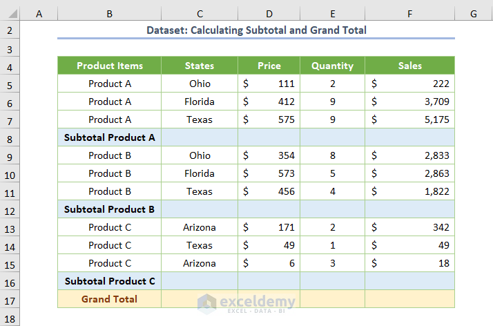
Let’s find the subtotals based on each group of products (i.e. Product A, Product B, and Product C), and we’ve shifted the dataset to divide it based on the groups. We’ll also determine the grand total (in the F17 cell) for all groups of products.

Steps:

Insert the SUBTOTAL function.
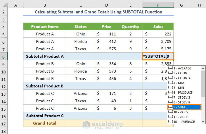
While entering the formula, you’ll see some groups of functions. From there, you need to select 9 as you’re going to compute the sum of the Sales.
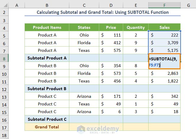
Select the cells (F5:F7) of Product A as the reference input.
The formula for the F8 cell will look like the following:

=SUBTOTAL(9,F5:F7)

Here, the SUBTOTAL function returns the sum values of the Sales in the case of Product A.

The following image displays the formula from the sample dataset.

Press Enter and copy-paste the formula (with Ctrl + C to copy and Ctrl + V to paste) to cells F12 and F16.

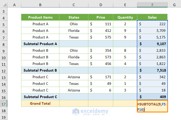
Insert the following formula in F17:

=SUBTOTAL(9,F5:F16)

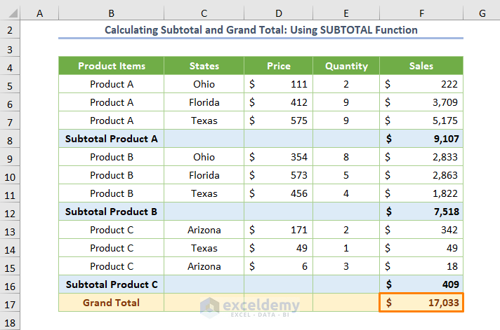
The function automatically excludes the computed subtotal of Products A, B, and C.

The output will be as follows.

Method 2 – Using the SUM Function

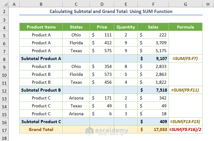
Here’s the formula for computing subtotal for Product A.

=SUM(F5:F7)

Copy and paste the formula for Product B and Product C.
The formula for calculating the grand total is:

=SUM(F6:F16)/2

The SUM function returns all the sum values. When I divided it by 2, it would return the actual grand total as subtotal values are available there.

Read More: How to Insert Subtotals in Excel

Method 3 – Utilizing the Subtotal Feature to Make a Subtotal and Grand Total

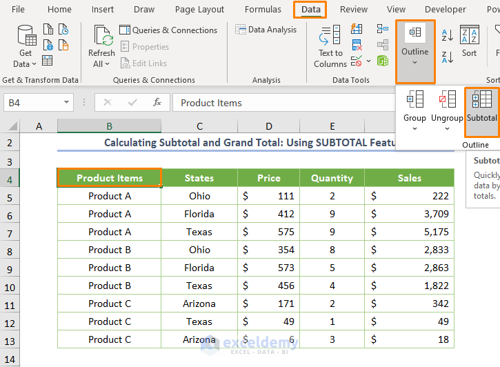
Select the dataset and keep the cursor over any cell within the dataset.
Go to the Data tab and the Data Tools ribbon, then click on the drop-down list for Outline and choose the Subtotal feature.

You’ll see a dialog box named Subtotal. Pick the Product Items from the drop-down list of the At each change in: option.
Put the Sum function in the function box and check Sales (from the options of Add subtotal to).
Check the box before Replace current subtotals and Summary below data options (these should be checked by default).

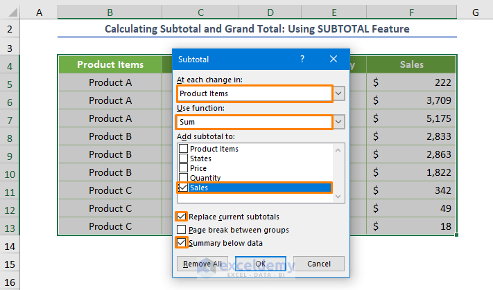
You’ll get the subtotal and grand total together after pressing OK.

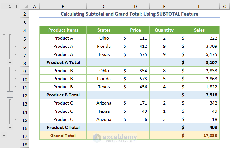
If you want to display only the Grand Total, just click over the 1 (located on the upper-left side as depicted in the following image).

Similarly, if you want only to represent the subtotal and grand total instead of the entire dataset, click over 2.

Method 4 – Use a Pivot Table to Get a Subtotal and Grand Total

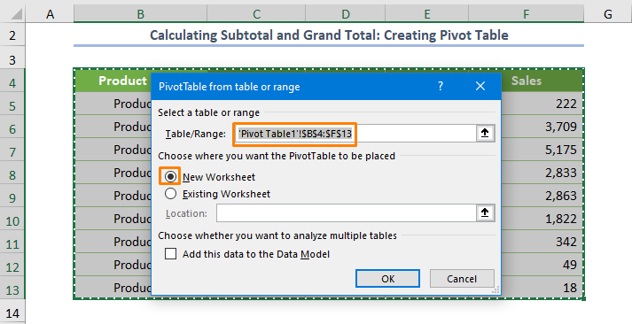
Select the entire dataset and pick the From Table/Range option by clicking over the drop-down list of the Pivot Table in the Insert tab.

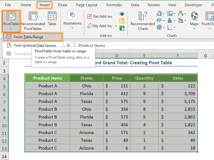
Press OK (keep the default options).

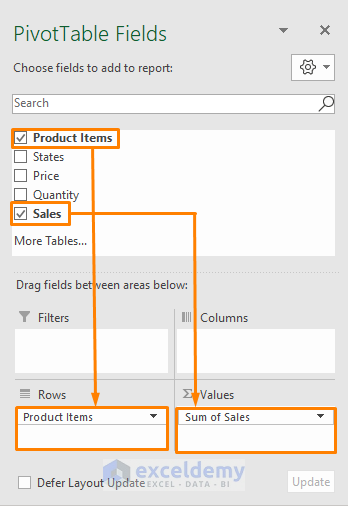
Drag the Fields to their relative areas. For the example, the Product Items go to Rows area and Sales to Values area.

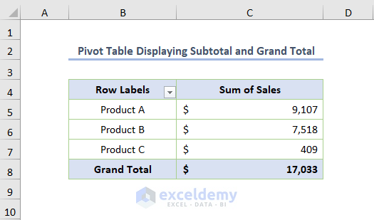
You’ll get the following output where the C5, C6, and C7 cells show the subtotal of Product A, B, and C respectively. The C8 cell displays the Grand Total.