[Fixed!] Missing Gridlines in Excel When Printing (5 Solutions)

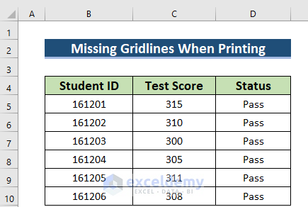
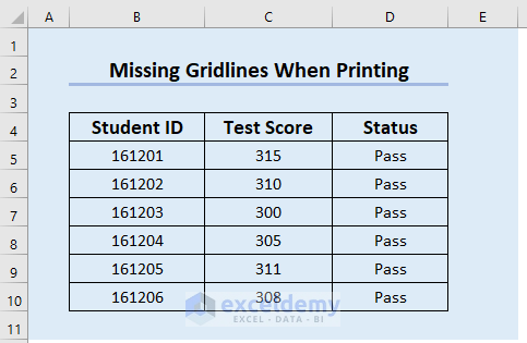
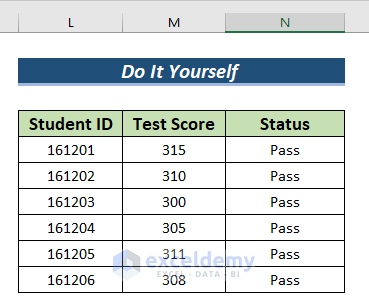
We will describe 5 possible ways to fix missing Gridlines in Excel when printing. We’ll use a sample data set named Missing Gridlines When Printing. It contains 3 columns: Student ID, Test Score, and Status. The dataset is given below.

Fix 1 – Using the Page Layout Ribbon in Excel

Solution:

• Open your worksheet in Excel.
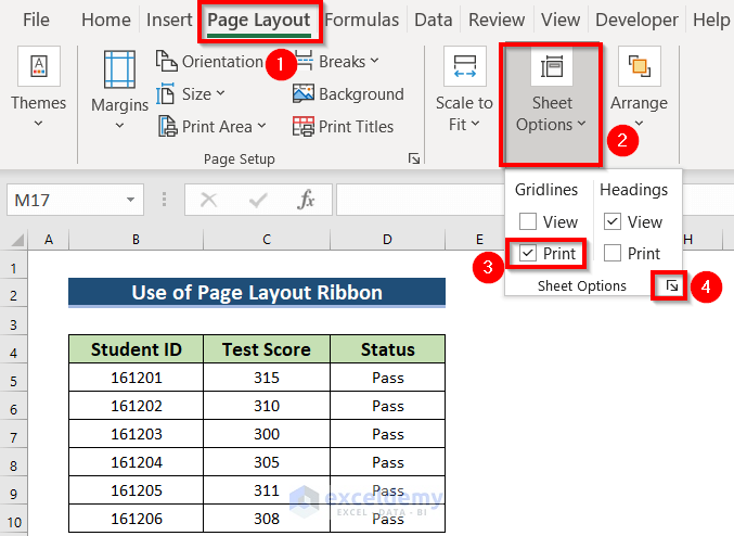
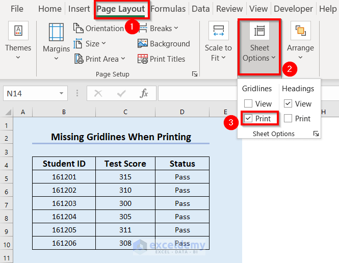
• Go to the Page Layout ribbon. Here, you can also use Excel keyboard shortcuts Alt + P to go to the Page Layout ribbon.
• From the Sheet Options, checkmark Print under Gridlines option.
• Click on the Drop-Down Arrow to see the printing draft.

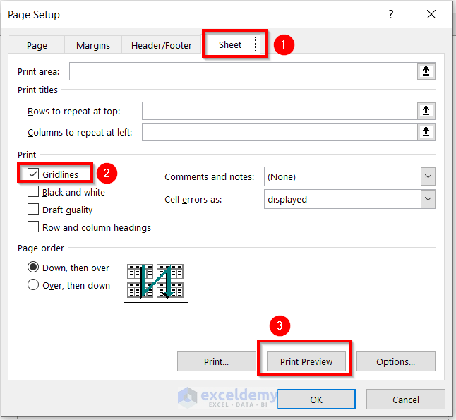
• A dialog box named Page Setup will appear.
• Ensure that the Gridlines option of the Print section under Sheet is marked.
• Select the Print Preview option from the Page Setup dialog box.

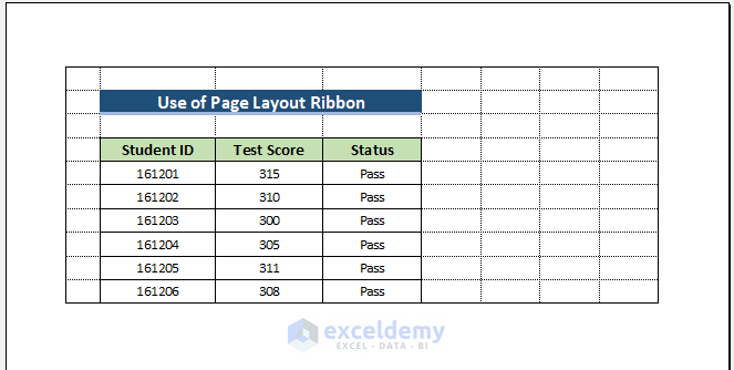
• You will see the following page layout which includes the Gridlines.

Fix 2 – Changing Gridline Color

Solution:

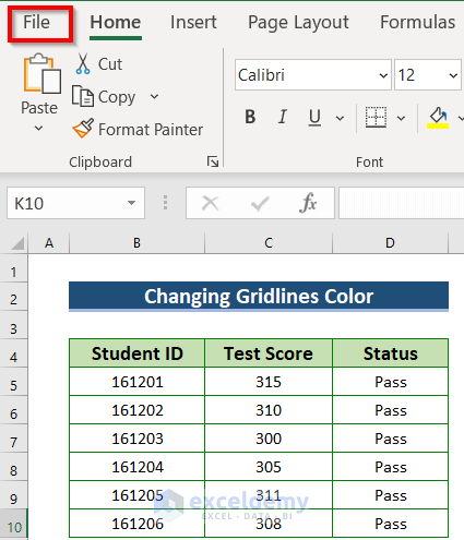
• Go to the File ribbon.

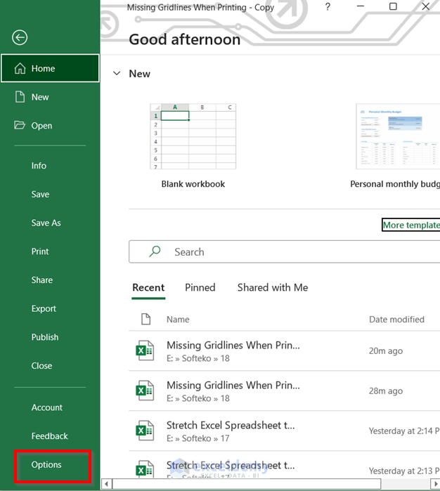
• Select the Options command.

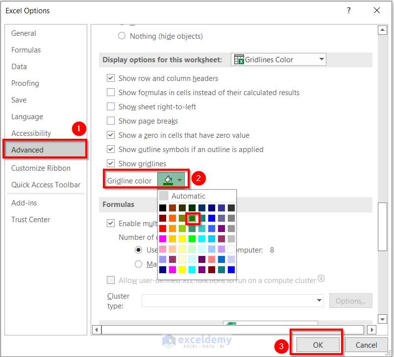
• A dialog box named Excel Options will appear.
• Select the Advanced tab..
• For Gridline color, choose your preferred color. We have chosen green.
• Press OK to confirm the changes.

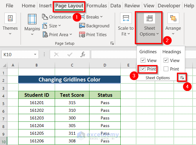
• Go to the Page Layout ribbon.
• From the Sheet Options, check Print under Gridlines.
• Click on the Drop-Down Arrow to see the printing draft.

• A dialog box named Page Setup will appear. Select the printing area.
• From the Sheet command in the Page Setup dialog box, go to Drop-Down Arrow which is adjacent to the Print area.

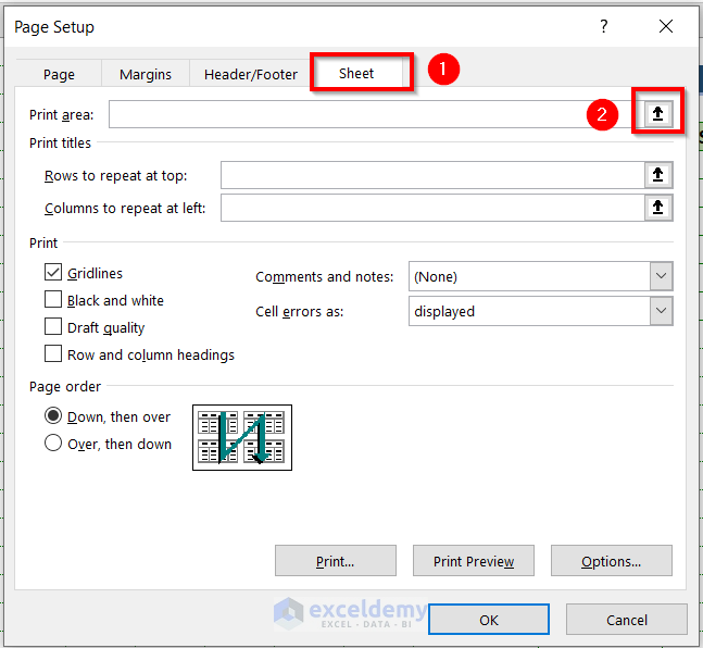
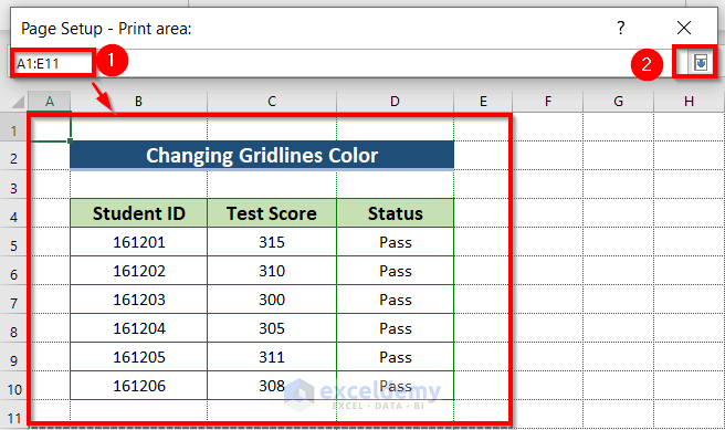
• Select the data up to which you want to print. We have selected the data range A1:E11.
• Click on the Drop-Down Arrow to go back to the whole Page Setup dialog box.

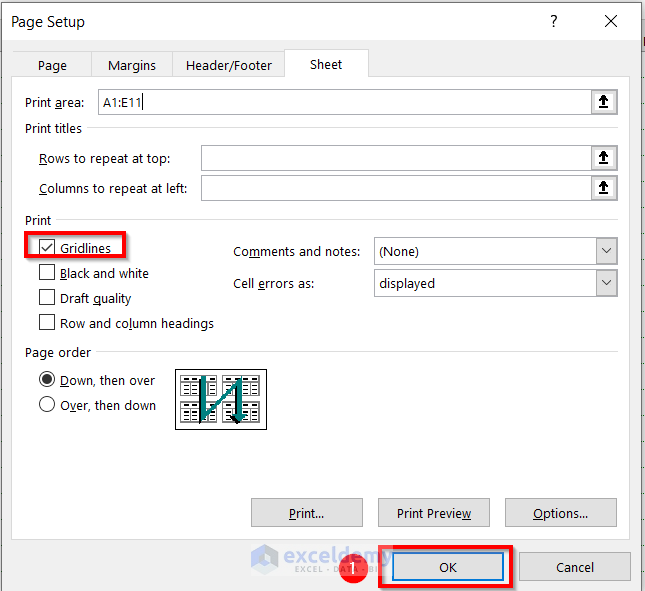
• Ensure that the Gridlines option of the Print section is marked.
• Press OK to make the changes.

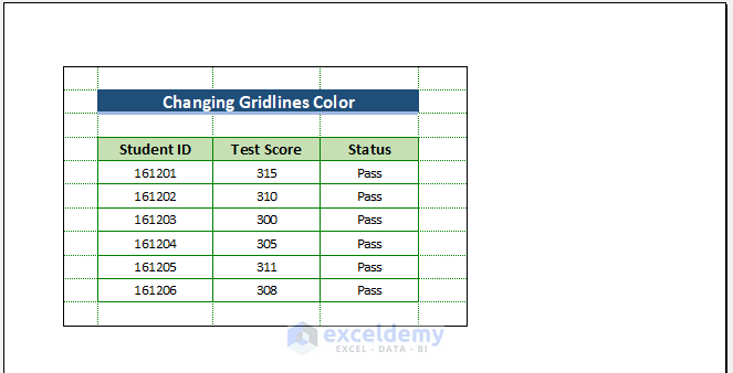
• If you go to the Print Preview option, you can see the following result which has visible Gridlines.

Fix 3 – Checking the Fill Color of the Printing Area

Here, the following dataset is filled with a background color.

We have marked Print under the Gridlines option.

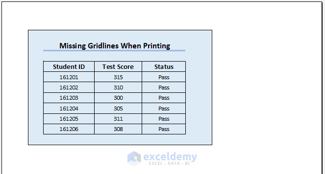
If you preview the printing draft then you will see no Gridlines in that paper.

Solution:

• Select the data range up to where you want to print. We have selected the range A1:E11.
• Go to the Home tab.

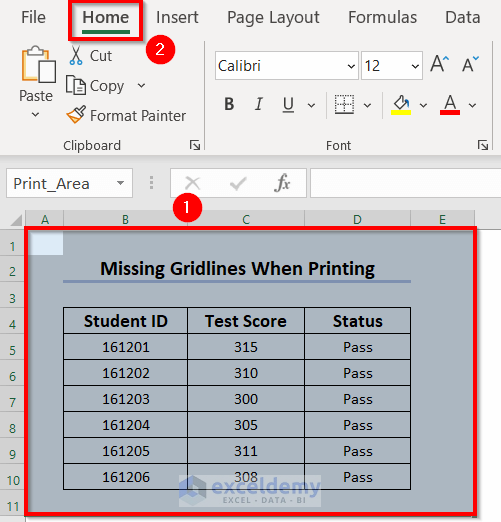
• From the Fill Color feature, choose No Fill.

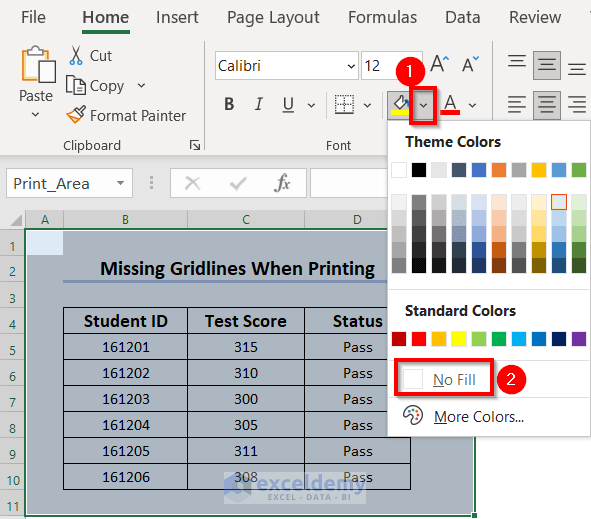
• You will see the following changes.

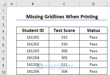
• Go to the Page Layout ribbon.
• From the Sheet Options, click Print under the Gridlines section.
• We have also changed the Title of the dataset to “Applying No Fill Color” in the following image.

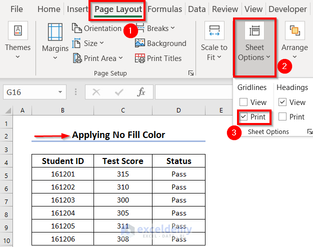
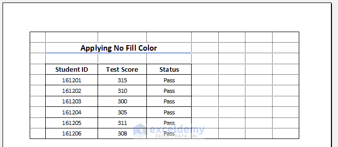
• If you preview the printing draft, you will be able to see the Gridlines. The result is given below.

Fix 4 – Removing Conditional Formatting

Solution:

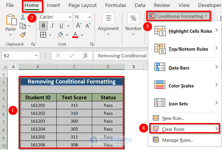
• Select the data range that is being printed.
• Go to the Home tab.
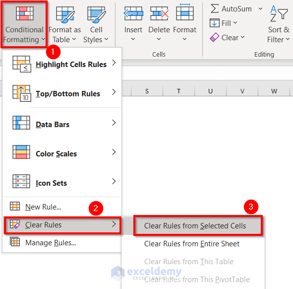
• From the Conditional Formatting section, choose Clear Rules.

• Select Clear Rules from Selected Cells.

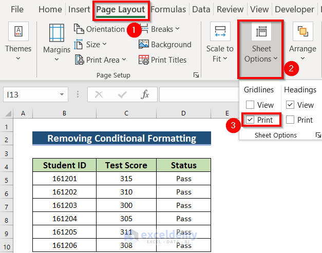
• Go to the Page Layout ribbon.
• From the Sheet Options, check Print under Gridlines.

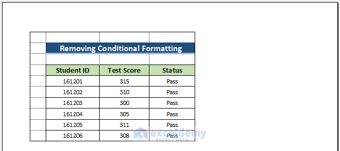
• If you preview the printing draft, you will be able to see the Gridlines. The result is given below.

Read More: How to Print Excel Sheet with Lines

Fix 5 – Using the Context Menu Bar to Format Cells

Solution:

• Select the data.
• Right-click.
• From the Context Menu Bar, select the Format Cells option.

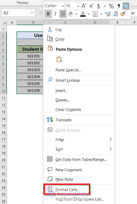
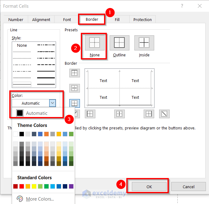
• A dialog box named Format Cells will appear.
• Go to the Border option.
• Select None.
• Alternatively, you can check whether the Color is Automatic. If the Color becomes White, change it to any visible colors.
• Press OK to make the changes.

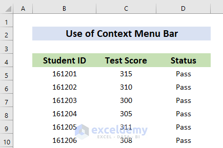
• You will see the following formatted cells.

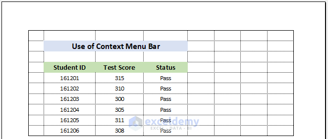
• If you preview the printing draft, you will be able to see the Gridlines. The result is given below.

Things to Remember

• Always, you must check the Print option under Gridlines to get the Gridlines in Excel while printing.

Practice Section

You can practice the explained methods by yourself in our practice workbook.

Download the Practice Workbook

Related Articles