How to Perform Mixed Integer Linear Programming in Excel

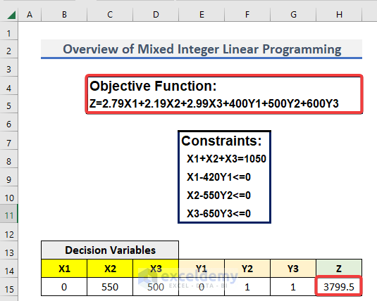
Here is an overview of mixed integer linear programming via the Solver.

Introduction to Mixed Integer Linear Programming

Mixed Integer linear programming is a type of mathematical method that consists of integer variables and linear objective functions and equations. The mixed-integer linear programming has both continuous and integer variables. With the help of linear programming, we can determine the minimum or maximum outcome of a given problem with some conditions. It is a tool that can be used to achieve a way to apply limited resources in the best possible manner. It uses:

• Decision Variables: The decision variables that minimize or maximize the objective function.
• Objective Function: This is a function that helps us to determine the decision variables. It expresses the relation between the result and the variables.
• Constraints: Constraints are also functions that denote different conditions on possible solutions.

Perform Mixed Integer Linear Programming in Excel: Step-by-Step Procedures

We have to set your objective function and the constraints.

Step 1 – Insert Details

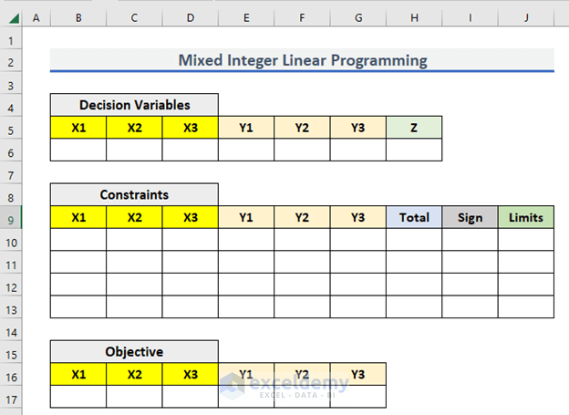
• Create three separate tables like below. The tables should include:
  • Decision Variables
  • Constraints
  • Objective

Step 2 – Load the Solver Add-in in Excel

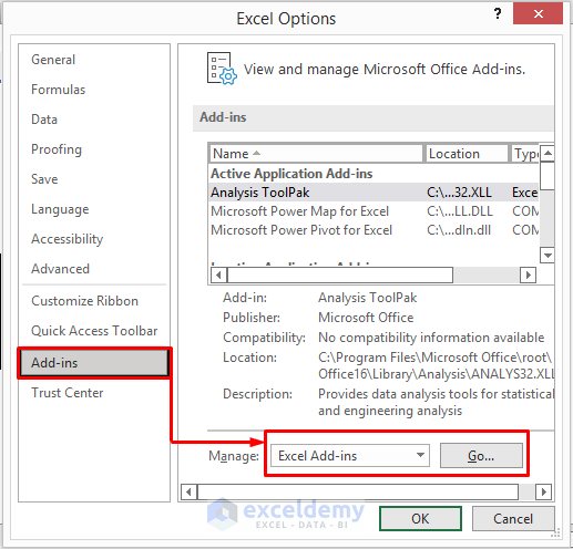
• Click on the File tab.

• Select Options.

• This will open the Excel Options.
• Select Add-ins.
• Select Excel Add-ins and click on Go in the Manage.

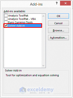
• The Add-ins message box will pop up.
• Check Solver Add-in and select OK from the message box.

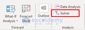
• You will see the Solver feature in the Analysis section of the Data tab.

Read More: How to Use Excel Solver for Linear Programming

Step 3 – Type the Mixed Coefficients of Objective Function and Constraints

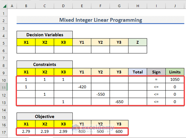
• Write down the coefficients of the objective function in the B17:G17 range.
• Input the coefficients of the constraints in the B6:J13 range.
• Keep the Total column empty for now.
• Your worksheet should look like this.

Step 4 – Calculate the Totals

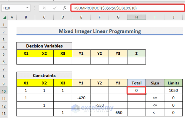
• Go to H10 and enter the following formula

• Press Enter to get the output.

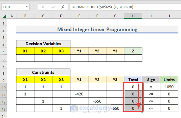
• Use the Fill Handle to AutoFill up to H13.

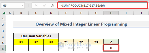
Step 5 – Measure the Dependent Variable of Objective Function

• Go to H6 and insert the following formula.

• Hit Enter.

Step 6 – Apply the Solver Add-in

• Go to the Data tab.
• Select Solver.

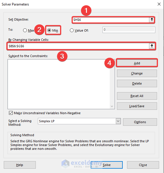
• A Solver Parameters window will appear.
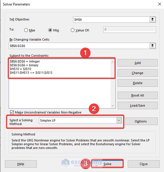
• Set the objective H6 to be minimum.
• Set the variables that Excel is going to change.
• Select Add to set the constraints.

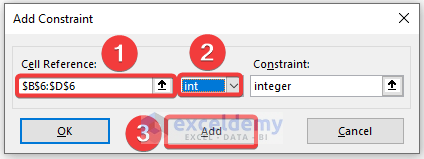
• After clicking Add, an Add Constraint box will appear.
• Set the Cell Reference and the condition from the drop-down list.
• Click Add.

• Excel has added a constraint.

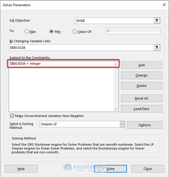
• Add other constraints.
• Select a solving method.
• Click Solve.

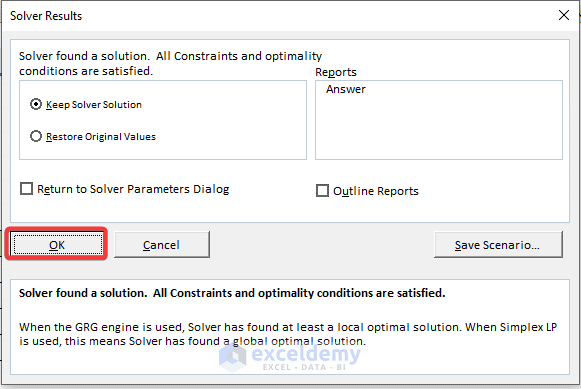
• The Solver Result box will appear.
• Click OK.

Step 7 – Show Final Output

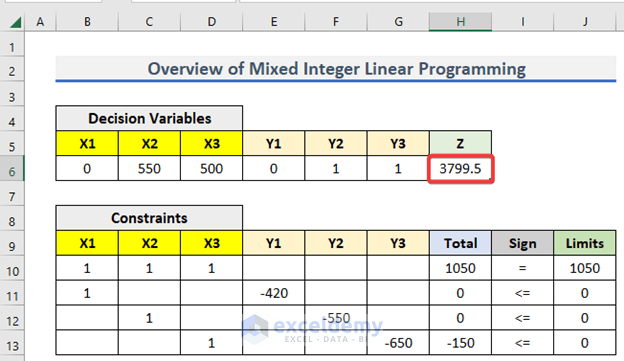
After clicking OK, Excel will solve the problem for you. The outputs are shown below.

Read More: How to Find Optimal Solution in Linear Programming Excel

Download the Practice Workbook

Related Articles 

• Calculate Shadow Price Linear Programming in Excel
• How to Solve Integer Linear Programming in Excel
• How to Do Linear Programming in Excel
• How to Graph Linear Programming in Excel 
• How to Do Linear Programming with Sensitivity Analysis in Excel
• How to Solve Blending Linear Programming Problem with Excel Solver

<< Go Back to Excel Linear Programming | Solver in Excel | Learn Excel