We need four main components in a money management Excel sheet for trading:
- “Key Factors”
- “Date for Trades”
- “Probable Trades (Qty Calculation)”
- “Actual Trades”
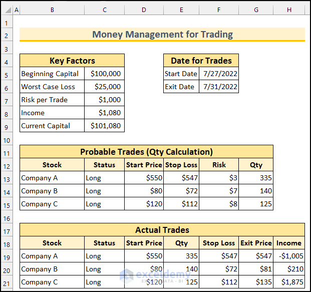
Here is the final snapshot of our money management Excel sheet for trading.
Step 1 – Inputting Key Factors for Trading
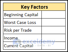
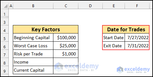
- Insert the following key factors, one in each cell:
- “Beginning Capital” → the initial investment from an individual to start this trading.
- “Worst Case Loss” → the maximum amount of loss that a person can suffer, which ranges from 20% to 30%.
- “Risk per Trade” → this is the amount of risk that will be taken for each trade and it should be less than 2%.
- “Income” → the profit or loss generated from actual trading.
- “Current Capital” → summation of the initial capital and the profit or loss amount.
- Type the amount of beginning capital.
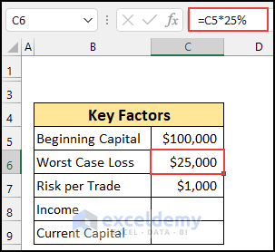
- The “worst case loss” is equal to 25% of the “beginning capital”. The industry’s standard risk ranges from 20% to 30%. Use the following formula in cell C6.
=C5*25%
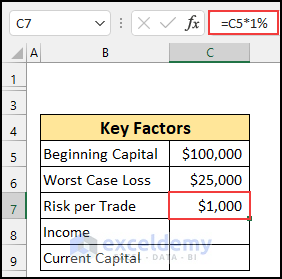
- We keep our risk to 1%. This risk should be between 0.5% and 2%. If you take less than 0.5%, then your risk will be too low. Use this formula in cell C7.
=C5*1%
- Add the start and exit dates for your trade.
- Input the values for the “Income” and “Current Capital” cells.
Step 2 – Trade Quantity Calculation
- Insert the following fields:
- Stock → List the company you want to buy or sell.
- Status → Short or Long.
- Start Price → The price of the stock on the starting date.
- Stop Loss → To limit your loss.
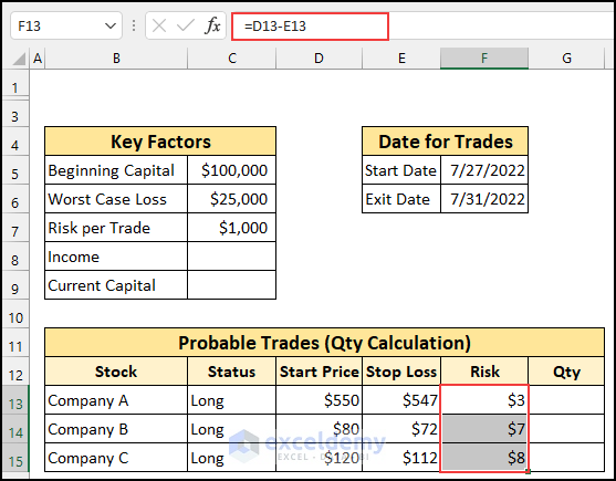
- Risk → The difference between the “Start Price” and the “Stop Loss”.
- Qty → We will calculate this from these values and the risks from the first step.

- Input the details of the probable trades.

- Use this formula in cell F13 to find the risks related to Company A’s stock.
=D13-F13
- Our values are higher in the Start Price column. If yours are not, you can use this formula to get positive values.
=ABS(D13-F13)
- AutoFill the formula into the rest of the cells.
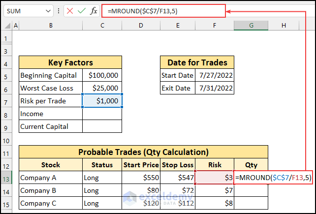
- Use this formula in cell G13.
=MROUND($C$7/F13,5)
This formula divides the “Risk per Trade” amount by the “Risk of each company’s stock”. Then, it rounds up or down to the nearest multiple of 5.
- Press Enter and then AutoFill the formula to the rest of the cells.
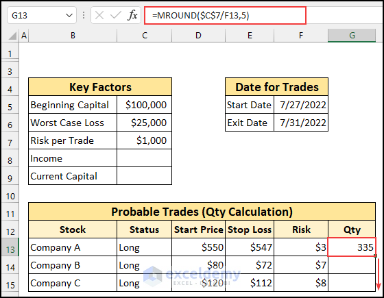
- Here’s the probable trades table.

Step 3 – Adding Actual Trades
- Insert the following data into the sheet:
- Stock → List the company you want to buy or sell, taken from the last step.
- Status → Short or Long, taken from the last step.
- Start Price → The price of the stock on the starting date, taken from step 2.
- Qty → obtained from step 2.
- Stop Loss → To limit your loss, obtained from the last step.
- Exit Price → The selling price of the stocks.
- Income → Profit or loss gained from selling the stocks, which we will calculate using a formula.

- Input in the relevant data.

- Use the following formula in cell H19.
=IF(C19="Long", G19*E19-D19*E19, (D19*E19-G19*E19))
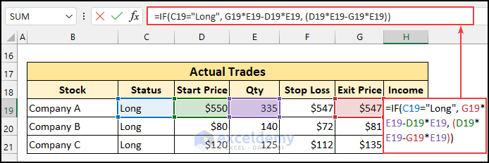
- Press Enter and AutoFill the formula into the rest of the cells.
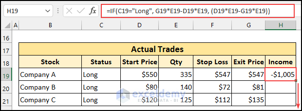
Formula Breakdown
- The logical_test of this formula is C19 = ”Long”. If this is true, then the first part of the formula executes. Alternatively, the second part of the formula will be executed.
- Our formula reduces to → IF(TRUE,-1005,1005)
- Output: -1005.
- As this is true so the first part of the formula will be executed.

Step 4 – Calculating the Total Income from Trades
- Use the following formula in cell C8. This formula adds all the profit or loss from all the trades
=SUM(H19:H21)
- Press Enter.
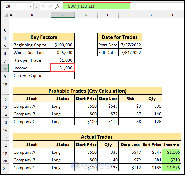
- We will find the amount of Current Capital by using this formula in cell C9.
=C5+C8
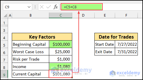
- Here’s the finalized money management sheet for trading.

Download the Free Template
<< Go Back to Money Management | Finance Template | Excel Templates
Get FREE Advanced Excel Exercises with Solutions!

