Below is a dataset with the examination records of some school students. Our objective is to find the overall result of each student based on their results in Physics and Chemistry.
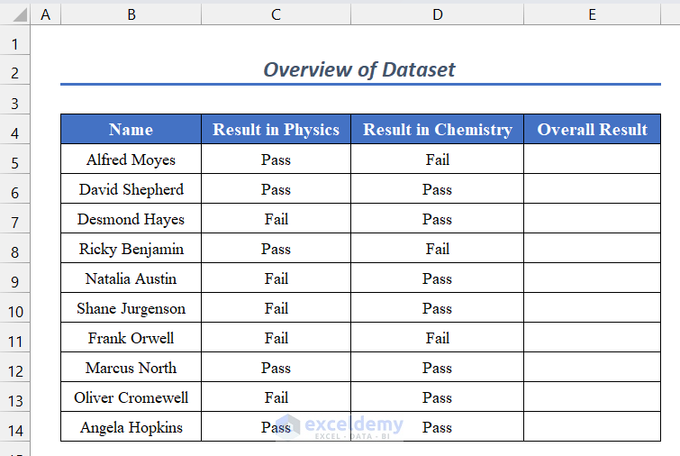
Method 1 – Using the AND Condition with IF Function for Case-Insensitive Match
Steps:
- Select cell E5.
- Enter the following formula in the cell:
=IF(AND(C5="pass",D5="pass"),"Pass","Fail")
- Press Enter.
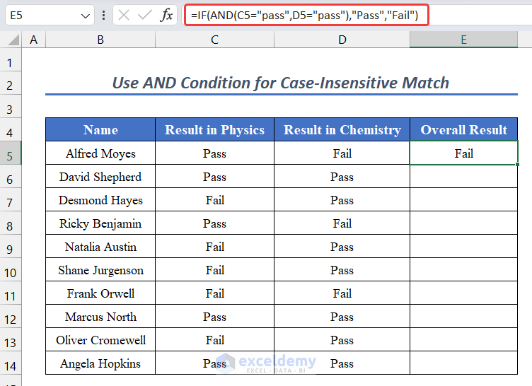
- Drag the AutoFill Handle to copy this formula to the rest of the cells.
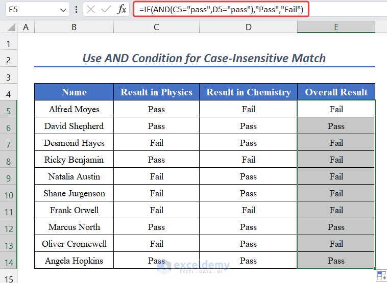
You will get the result for all the cells.
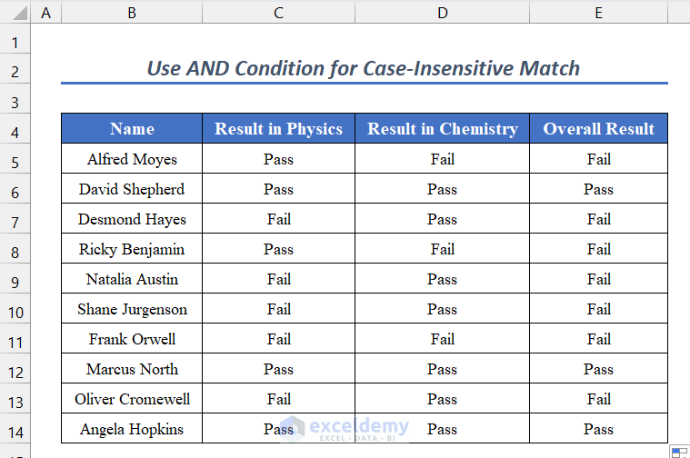
Code Breakdown
- The IF function matches case-insensitive matches by default. So whether you use C4=“pass” or C4=“Pass” doesn’t matter here.
- AND(C4=”pass”,D4=”pass”) returns TRUE only if both conditions are TRUE. Otherwise, it returns FALSE.
- Therefore, IF(AND(C4=”pass”,D4=”pass”),”Pass”,”Fail”) will return “Pass” only if he/she passes in both the subjects, otherwise, it will return “Fail”.
Method 2 – Applying the AND Condition with the IF Function for Case-Sensitive Match
Steps:
- Select cell E5.
- Enter the following formula in the cell:
=IF(AND(EXACT(C5,"Pass"),EXACT(D5,"Pass")),"Pass","Fail")
- Press Enter.
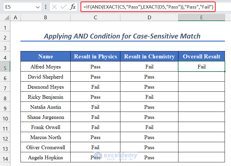
- Drag the AutoFill Handle to copy this formula to the rest of the cells in column E.
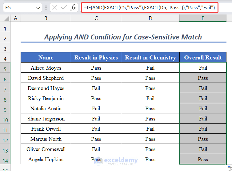
You will see all the results will appear in our desired column.

Code Breakdown
- The EXACT function works with case-sensitive matches. So you have to use exactly EXACT(C4,”Pass”).
- EXACT(C4,”pass”) will not work here. It will return FALSE. You can test it yourself.
- The rest is like the previous formula. IF(AND(EXACT(C4,”Pass”),EXACT(D4,”Pass”)),”Pass”,”Fail”) will return “Pass” only if there is “Pass” in both the subjects.
Method 3 – Utilizing the OR Condition with the IF Function for Case-Insensitive Match
Steps:
- Select cell E5.
- Enter the following formula in the cell:
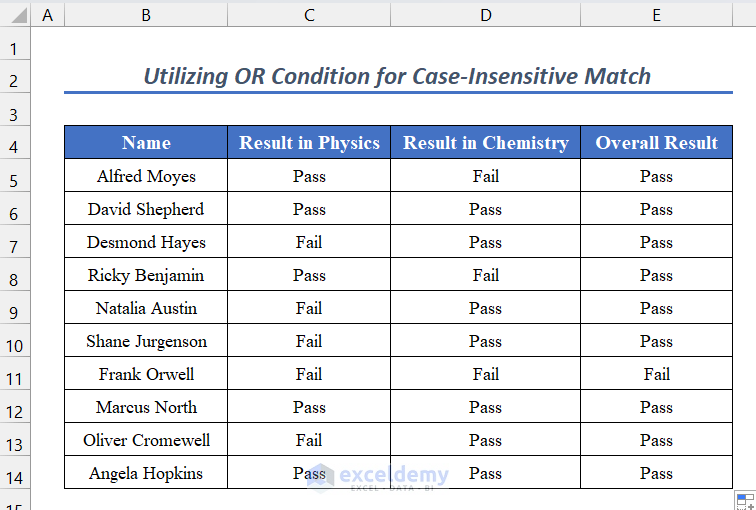
=IF(OR(C5="pass",D5="pass"),"Pass","Fail")
- Press Enter.
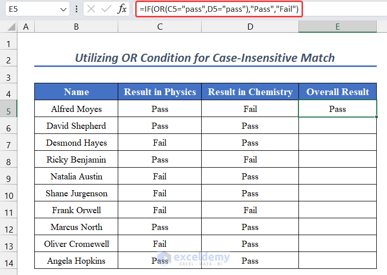
- Drag the AutoFill Handle to copy this formula to the rest of the cells.
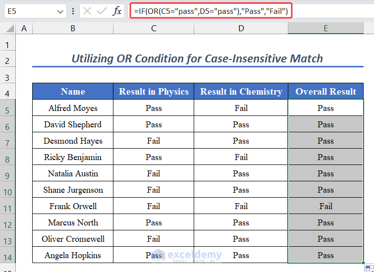
You will figure out the results.
Code Breakdown
- The IF function matches case-insensitive matches by default. So whether you use C4=“pass” or C4=“Pass” doesn’t matter here.
- OR(C4=”pass”,D4=”pass”) returns TRUE if at least one of the conditions is TRUE. Otherwise, it returns FALSE.
- Therefore, IF(OR(C4=”pass”,D4=”pass”),”Pass”,”Fail”) will return “Pass” if he/she passes in at least one subject, otherwise it will return “Fail”.
Method 4 – Applying the OR Condition with the IF Function for Case-Sensitive Match
Steps:
- Select cell E5.
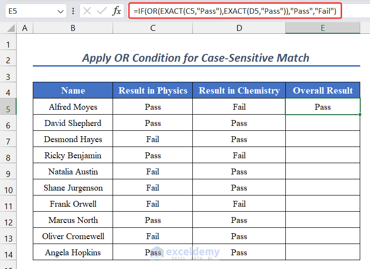
- Enter the following formula in the cell:
=IF(OR(EXACT(C5,"Pass"),EXACT(D5,"Pass")),"Pass","Fail")
- Press Enter.
- Drag the AutoFill Handle to copy this formula to the rest of the cells.
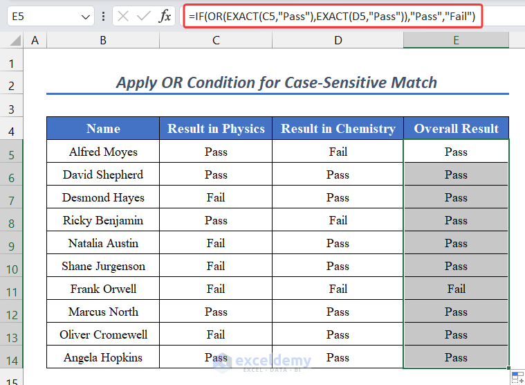
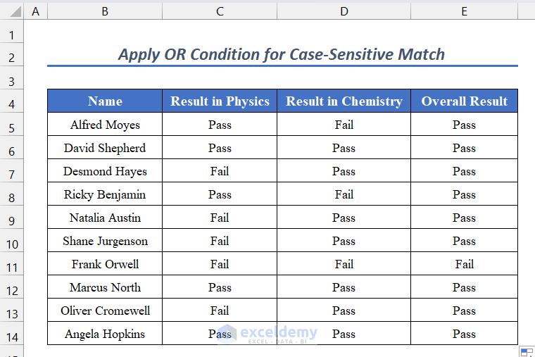
You will see the result in column E.
Code Breakdown
- The EXACT function works with case-sensitive matches. So you have to use exactly EXACT(C4,“Pass”).
- EXACT(C4, “pass”) will not work here. It will return FALSE. You can test it yourself.
- The rest is like the previous formula. IF(OR(EXACT(C4,”Pass”),EXACT(D4,”Pass”)), ”Pass”,”Fail”) will return “Pass” if there is “Pass” in at least one subject.
Method 5 – Using Nested IF Statements for Multiple Conditions
Steps:
- Select cell E5.
- Enter the following formula in the cell:
=IF(OR(EXACT(C5,"Pass"),EXACT(D5,"Pass")),"Pass","Fail")
- Press Enter.
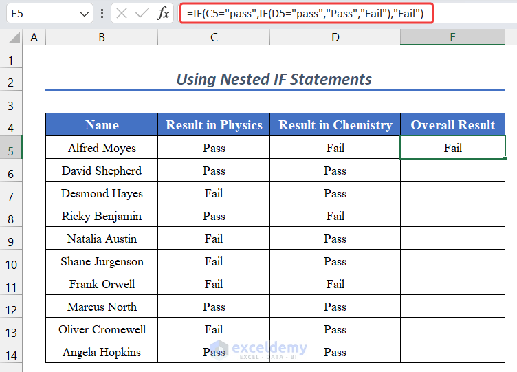
- Drag the AutoFill Handle to copy this formula to the rest of the cells.
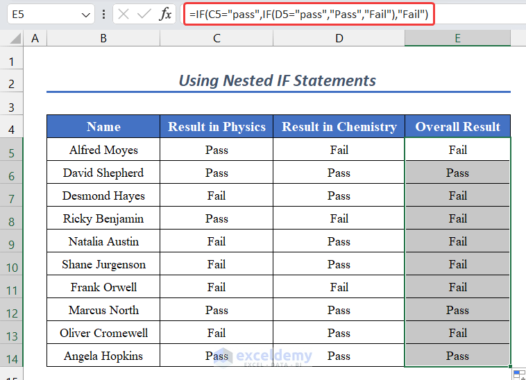
You will see the result.
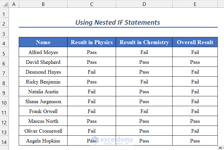
Code Breakdown
- Here, if the value in cell C4 is “Pass”, then it will move to see what the value in cell D4 is.
- If the value in cell D4 is also “Pass’, only then it will certify as “Pass”. Otherwise, it will certify as “Fail”.
- And the IF function returns a case-insensitive match. So C4=”pass” or C4=”Pass” really doesn’t matter here.
Read More: How to Use IF Function with Multiple Conditions in Excel
Method 6 – Multiplying the IF Statements with Array Formula for Condition Range
Steps:
- Select cell E5.
- Enter the following formula in the cell:
=IF(OR(EXACT(C5,"Pass"),EXACT(D5,"Pass")),"Pass","Fail")
- Press Enter.
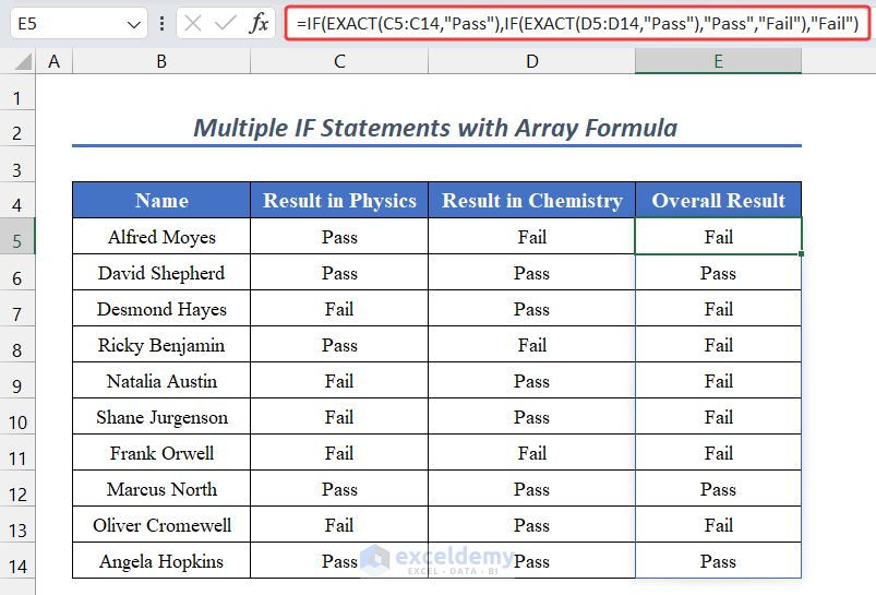
You will see the result in our desired area.
Code Breakdown
- Here, C4:C13 and D4:D13 are the two ranges of my criteria. You use your one.
- Here, we are opting for a case-sensitive match. If you want a case-insensitive match, use C4:C13=“Pass” and D4:D13=“Pass” instead.
- Press CTRL+SHIFT+ENTER to enter the formula unless you are in Office 365.
Download the Practice Workbook
Download this workbook for practice.
Related Articles
<< Go Back to Excel IF Function | Excel Functions | Learn Excel
Get FREE Advanced Excel Exercises with Solutions!


HI, I want to pull text from multiple sheets and ignore some specific text as blank or space. How to do it?
Example .
If sheet 1 has John in B2 and sheet2 has Jacob in B2 and i want an output in sheet3, where if sheet 2 has Jacob then ignore or blank.
Thanks for your query.
It’s kind of a complicated task to filter specific data from certain cells of different worksheets with certain condition. I have tried a possible simple solution to pull data from different sheets into one sheet using FILTER function.I have used the following dataset for filtering the rows having Geller as Last Name and replace the Geller word with blank.
I have used the following formula to fulfill the purpose.
=FILTER(IF(Dataset!B4:J17=”Geller”,””,Dataset!B4:J17),Dataset!C4:C17=”Geller”)
For further information related to Excel, you can send message via email. email id: [email protected]