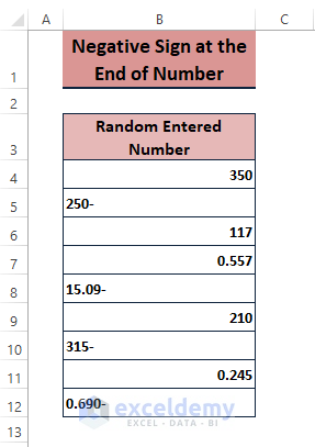
We have a column of random numbers as shown in the image below. We want to fix the negative signs’ positions in the entries.
3 Easy Methods to Move the Negative Sign at the End to the Left of a Number in Excel Error
Method 1 – Applying Formulas
Steps:
- Add a helper column adjacent to the existing column.
- Apply the below formula in the C4 cell.
=IF(RIGHT(B4,1)="-",SUBSTITUTE(B4,"-","")*-1,B4)In the formula, the IF function runs a logical_test using the Right function to find a negative sign (1 character). If the test outcome is TRUE, then the SUBSTITUTE function removes the end negative sign and multiplies it with -1. Otherwise, the entry remains unchanged.
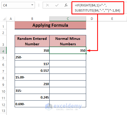
- Drag the Fill Handle to fill all cells.
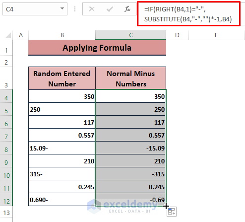
You can use an alternative formula to move negative signs:
=VALUE(IF(RIGHT(B4,1)="-",RIGHT(B4,1)&LEFT(B4,LEN(B4)-1),B4))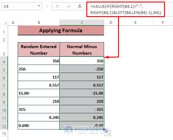
Read More: Excel Formula If Cell Contains Negative Number
Method 2 – Using the Text to Columns Feature
Steps:
- Select the entire range or column.
- Go to Data and the Data Tools section.
- Click Text to Columns.
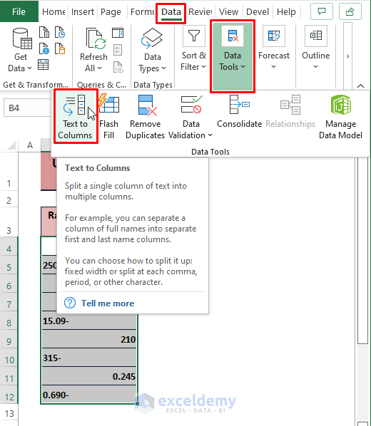
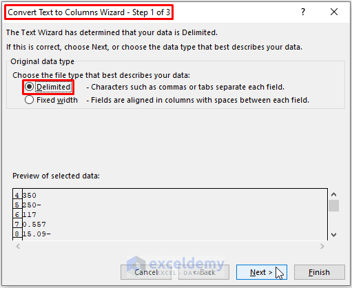
- This opens the Convert Text to Column Wizard -Step 1 of 3 window.
- Mark Delimited for Choose the file type that best describes your data.
- Click Next.
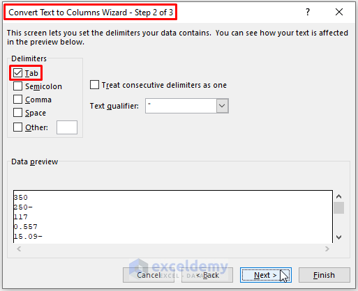
You’ll get the Convert Text to Column Wizard -Step 2 of 3 window.
- Tick Tab for Delimiters, then select Next.
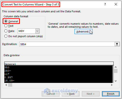
Another Convert Text to Column Wizard -Step 3 of 3 window appears.
- Click on Advanced.
The Advanced Text Import Settings dialog box appears.
- Tick the Trailing minus for negative numbers option.
- Click OK.
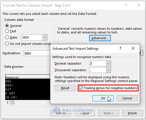
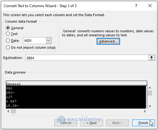
Excel returns to the Convert Text to Column Wizard -Step 3 of 3 window.
- Click on Finish.
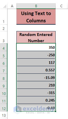
The trailing negative signs of the numbers get moved as shown in the below screenshot.
Read More: How to Put a Negative Number in Excel Formula
Method 3 – Using VBA Macro
Steps:
- Press Alt + F11 or move to the Developer tab and select Visual Basic to open the Microsoft Visual Basic window.
- Click Insert and select Module.
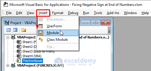
- Paste the following macro into the inserted Module.
Sub Fixing_NegativeSign()
Dim Rng As Range
Dim WrkRng As Range
On Error Resume Next
Set WrkRng = Application.Selection
Set WrkRng = Application.InputBox("Provide Range", "Exceldemy", WrkRng.Address, Type:=8)
Set WrkRng = WrkRng.SpecialCells(xlCellTypeConstants, xlTextValues)
For Each Rng In WrkRng
  xValue = Rng.Value
  If VBA.Right(xValue, 1) = "-" Then
  Rng.Value = "-" & VBA.Left(xValue, VBA.Len(xValue) - 1)
  End If
 Next
End Sub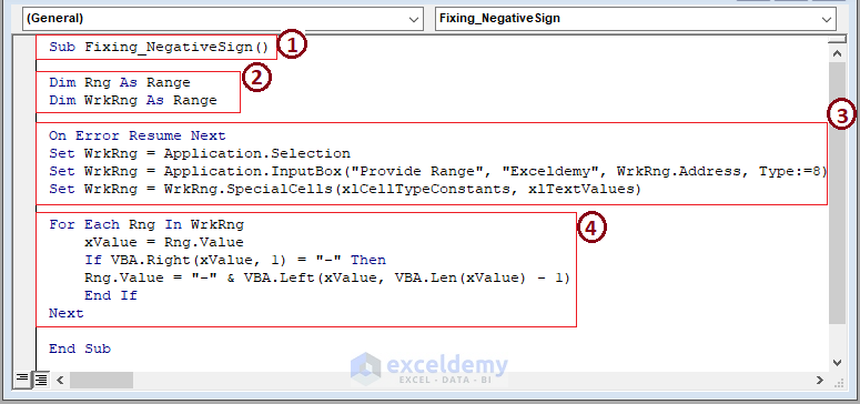
In the sections:
1 – begins the macro code by declaring the VBA Macro Code’s Sub name.
2 – declares the variable as Range.
3 – assigns the WrkRng variable to application selection, fetch an input box, and special cells.
4 – executes a VBA FOR loop to find the trailing minus signs using the VBA RIGHT function. Then the VBA LEFT function fetches the entries without negative signs. Inserting a minus using an Ampersand (&) deals with the negative signs.
- Hit F5 to run the macro.
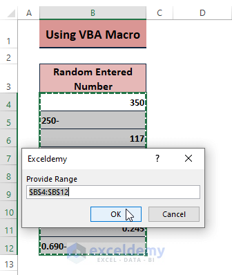
- Excel brings out the Provide Range command box.
- In the box, assign the desired range, then click on OK.
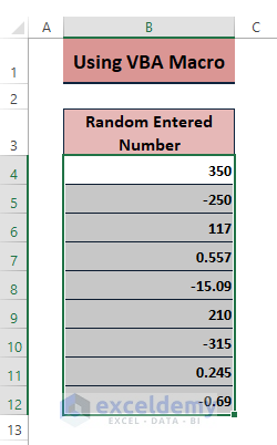
- Return to the worksheet.
Read More: Excel Formula to Return Zero If Negative Value is Found
Download the Excel Workbook
Related Articles
- Excel Negative Numbers in Brackets and Red
- How to Add Negative Numbers in Excel
- How to Put Parentheses for Negative Numbers in Excel
- How to Count Negative Numbers in Excel
- How to Apply Formula for Positive and Negative Numbers in Excel


