How to Paste Range Names in Excel (7 Ways)

In this article we will demonstrate some of useful ways to paste range names in Excel. Pasting range names can simplify working in Excel, particularly when making data tables or in formulas. We’ll use the following data table of Sales Records of a company to illustrate our methods.

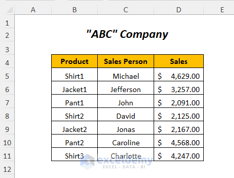
Method 1 – Using the Paste List Option to Paste a List of Defined Named Ranges

Here, we have named the three ranges of the three columns (Product, Sales Person, Sales) with the names product, person, and sales respectively. Let’s paste a list of these range names. 

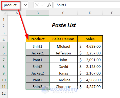
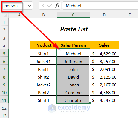
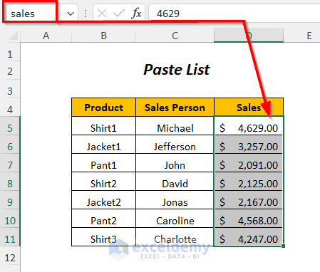
Steps:

• Make two columns named Range Name and Position in which to paste the list of the named ranges and their location.

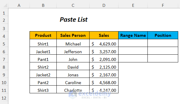
• Select the output cell E5.
• Go to the Formulas tab >> Defined Names >> Use in Formula >> Paste Names.

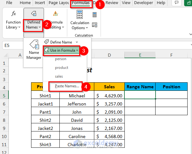
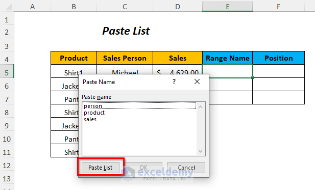
The Paste Name Wizard will pop up.

• Select the Paste List option.

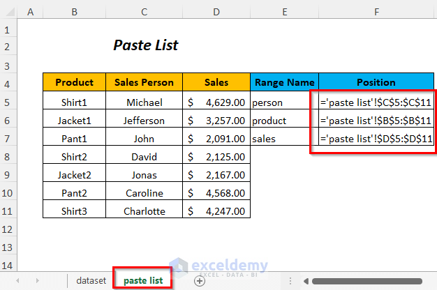
Result:

The list of the range names and their corresponding locations is returned.

Read More: How to Display Named Range Contents in Excel

Method 2 – Using the Paste Names Option to Paste Range Names

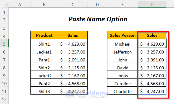
Here, we have two tables: the first has columns for Product and Sales, and the second has a Sales Person column. We have named the range of the Sales column as sales1. Let’s paste this range next to the Sales Person column in the second table using the Paste Names option.

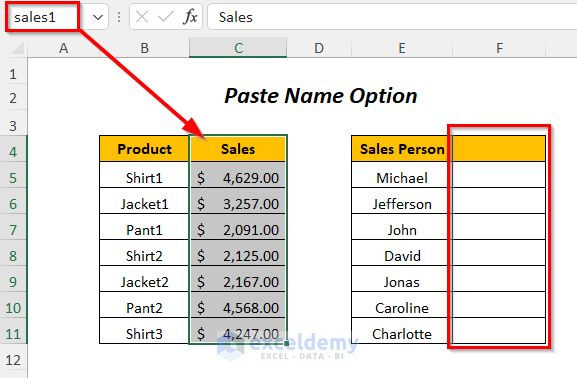
Steps:

• Select the output cell F4.
• Go to the Formulas tab >> Defined Names >> Use in Formula >> Paste Names

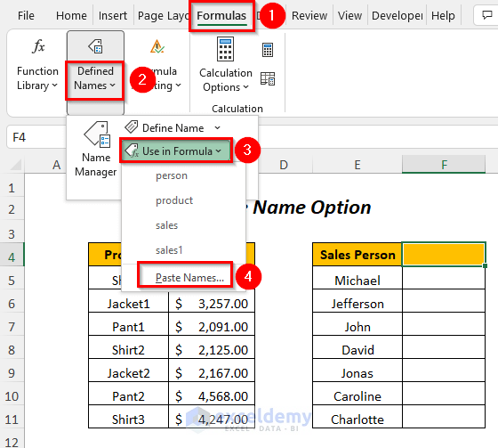
The Paste Name Wizard will pop up.

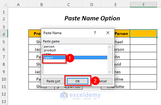
• Select the range name sales1.
• Click OK.

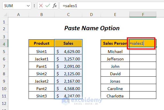
The following formula will appear in cell F4:

• Press ENTER.

Result:

The range name sales1 is pasted in Column F.

Things to Remember

The range name pasted here will work as a Dynamic Array, and individual cells in this array cannot be edited or deleted.

Read More: How to Delete Named Range in Excel

Method 3 – Pasting a Range Name in a Formula

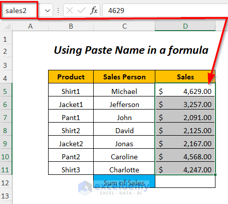
Suppose we have named the range in the column Sales as sales2. Let’s find the sum of sales by pasting the range name into the SUM function.

Steps:

• Select the output cell D12.
• Type the name of the function as follows:

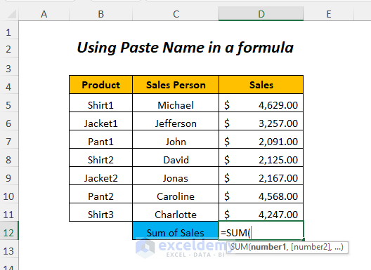
• Go to the Formulas tab >> Defined Names >> Use in Formula >> Paste Names.

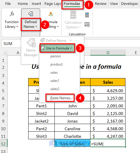
The Paste Name Wizard will pop up.

• Select the range name sales2.
• Click OK.

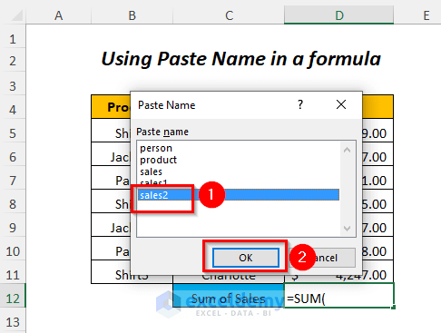
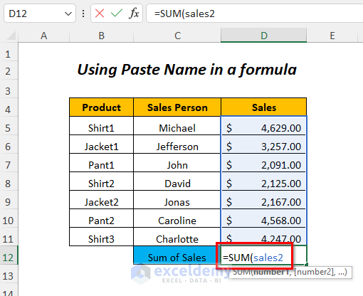
The range name will appear inside the function:

• Press ENTER.

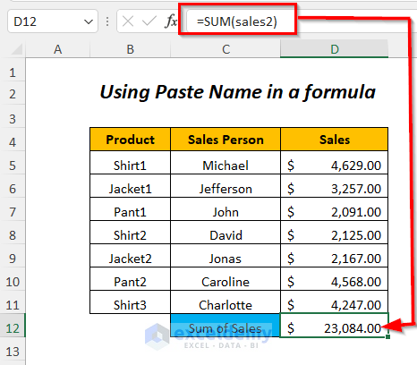
Result:

The Sum of Sales is returned in cell D12.

Read More: How to Name a Column in Excel

Method 4 – Using the Use in Formula List to Paste a Range Name in a Formula

Now we’ll paste the range name sales3 in our formula to find the sum of sales by using the Use in Formula list.

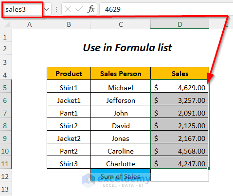
Steps:

• Select the output cell D12.
• Type the name of the function as follows:

• Go to the Formulas tab >> Defined Names group >> Use in Formula.
• Select the range name sales3 from the options in the Use in Formula list.

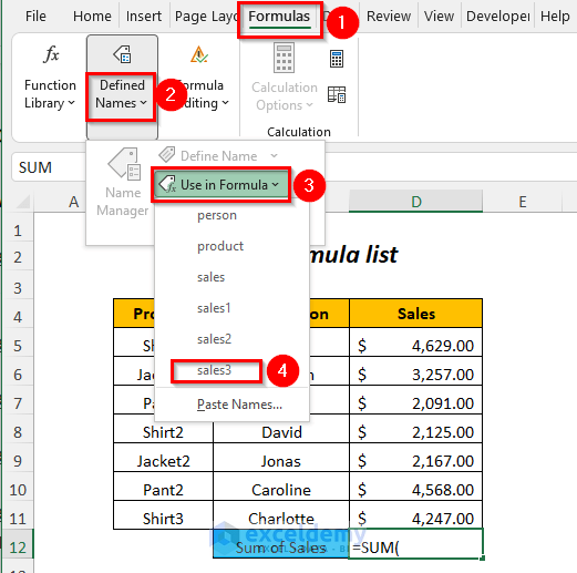
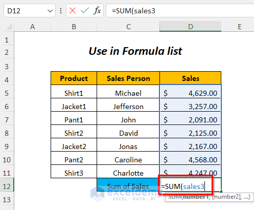
The range name will appear inside the function.

• Press ENTER.

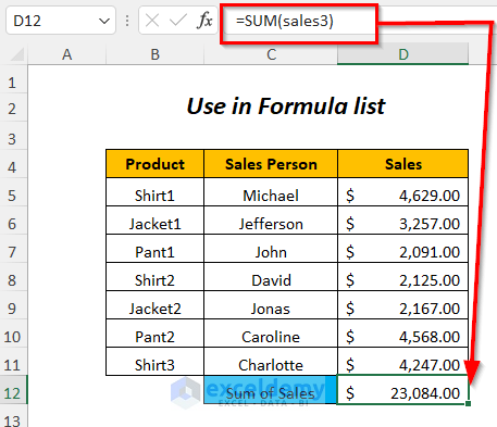
Result:

The Sum of Sales is returned in cell D12.

Method 5 – Using Formula Assistance to Paste Range Name in a Formula

We can also use Formula Assistance to paste the range name into our Sum of Sales formula.

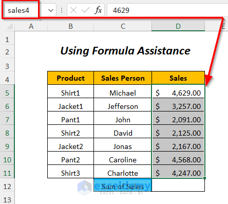
Steps:

• Select the output cell D12.
• Type the name of the function as follows:

• Start typing the name of the range, and a list of suggestions will appear.
• Select the name of the range from the list and press the TAB key.

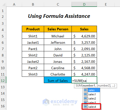
The range name will appear inside the function:

• Press ENTER.

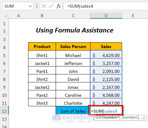
Result:

The Sum of Sales is returned in cell D12.

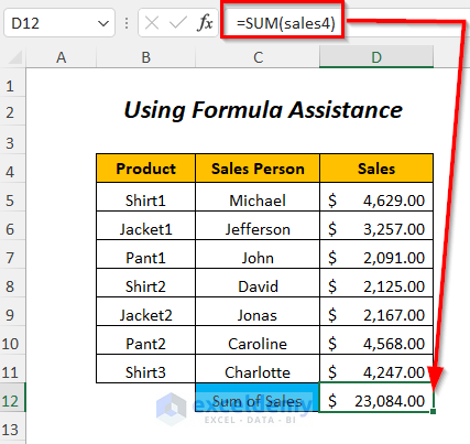
Method 6 – Using Apply Names in a Formula

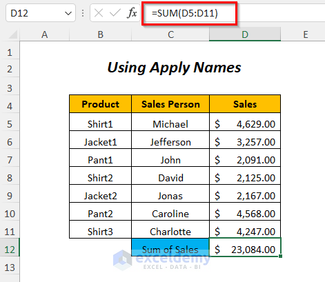
Suppose we’ve already used the SUM function to find Sum of Sales by using direct cell references instead of using the range name. We can change the cell references to the name of this range (sales5) by using the Apply Names option.

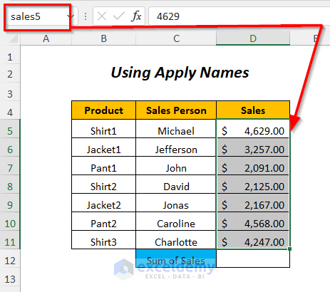
The formula we’ve used to find the Sum of Sales is as follows:

We will replace the range D5:D11 with its name, sales5.

Steps:

• Select the output cell D12.
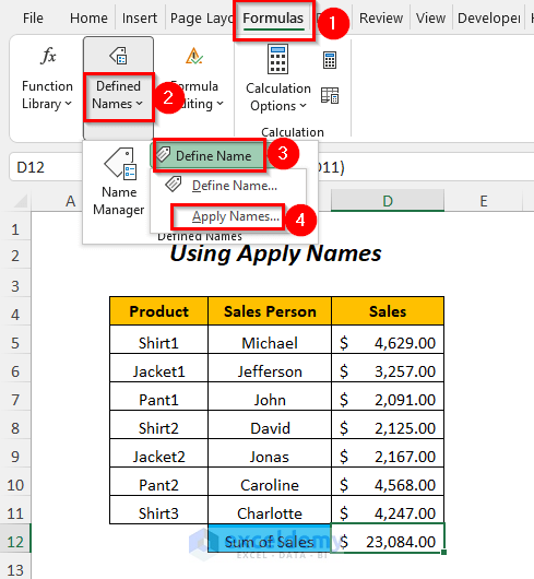
• Go to Formulas tab >> Defined Names group >> Define Name >> Apply Names.

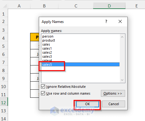
The Apply Names Wizard will pop up.

• Select the range name sales5.
• Click OK.

Result:

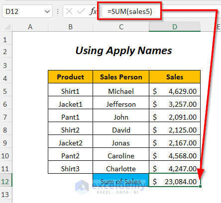
The cell references in the formula will be replaced with the range name sales5.

Read More: How to Edit Named Range in Excel

Method 7 – Using VBA Code

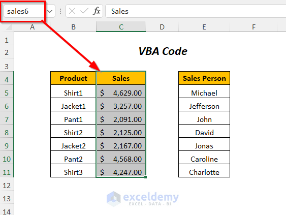
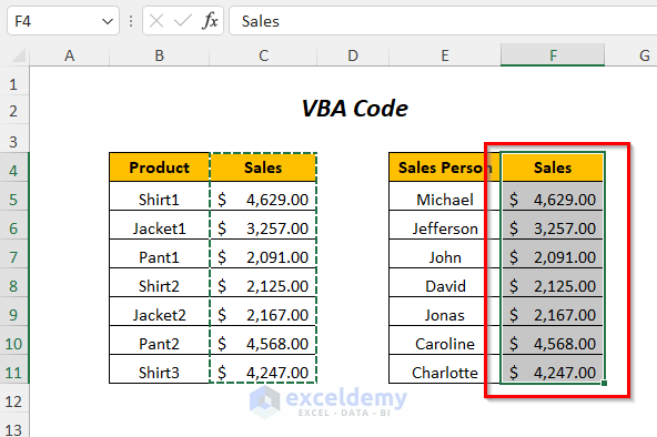
Suppose we have named the range of the Sales column as sales6 and now we want to paste this range adjacent to the Sales Person column in the second table.

We’ll accomplish this by using a VBA code.

Steps:

• Go to the Developer tab >> Visual Basic.

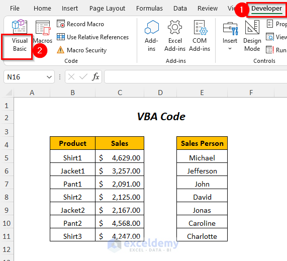
The Visual Basic Editor will open.

• Go to the Insert tab >> Module.

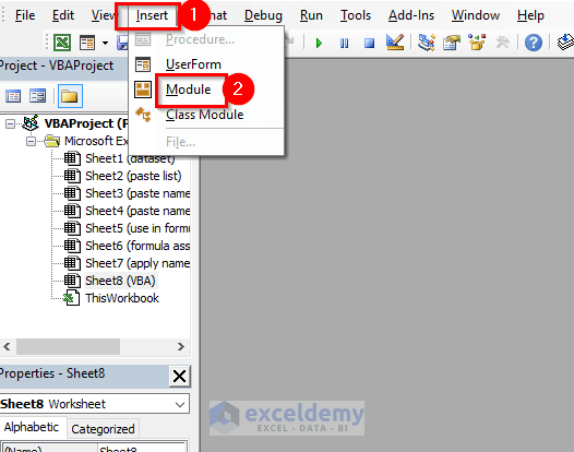
A Module will be created.

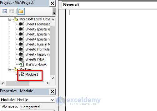
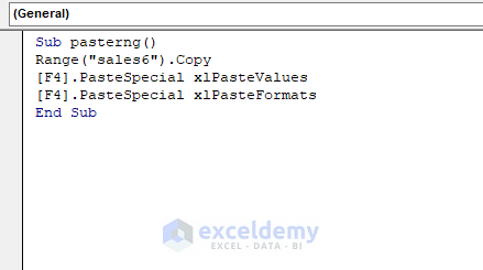
Enter the following code in the module window:

Sub pasterng()

    Range("sales6").Copy
    [F4].PasteSpecial xlPasteValues
    [F4].PasteSpecial xlPasteFormats

End Sub

Here, sales6 is the range name. We will copy it and paste the values with their formats into the cell range F4:F11.

• Press F5 to run the code.

Result:

The range with name sales6 is pasted in Column F.

Download Practice Workbook

Further Reading

• How to Find a Named Range in Excel
• How to Navigate to a Named Range in Excel
• How to Name a Group of Cells in Excel
• How to Change Scope of Named Range in Excel
• How to Delete All Named Ranges in Excel

<< Go Back to Named Range | Excel Formulas | Learn Excel