Personal Loan EMI Calculator Excel Format (2 Suitable Examples)

Example 1 – Applying Conventional Formula

We have our principal amount, interest and tenure to calculate the monthly interest.

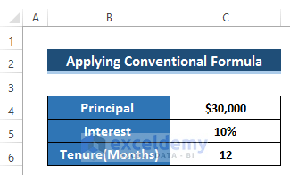
Steps:

• Select cell C7.

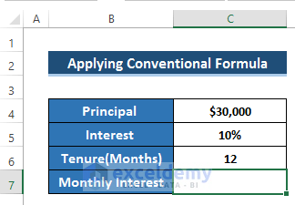
• The monthly interest is the ratio of the interest rate and the total monthly.
• Enter the following formula in the formula box.

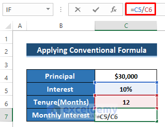
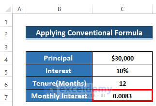
• Press Enter to apply the formula.

• Take this into a single worksheet where you would like to create the EMI calculator.
• Create some row headers including EMI, interest, principal and principal remaining.
• The principal remaining is the total amount of loan that you take.
• After 12 months, the principal remaining must be zero. That’s the ultimate target.

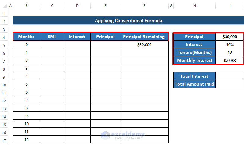
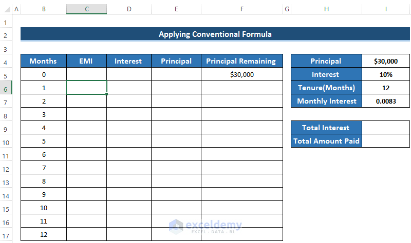
• To calculate the EMI in the first month, select cell C6.

• To calculate the EMI, enter the conventional formula in the formula box.

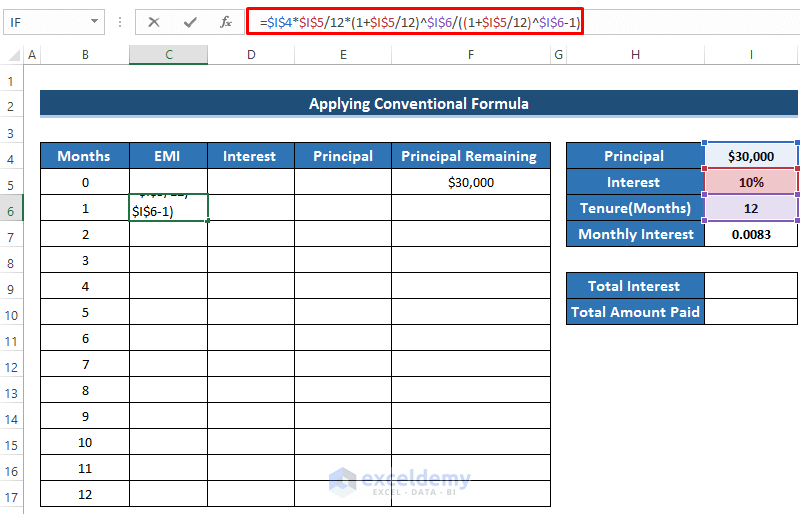
• Press Enter to apply the formula.

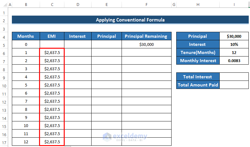
• The most important thing to remember is that you need to have the same EMI for every value. If you look at the formula, you will find all the cells are made constant by using the ($) sign.
• Drag the Fill handle icon down the column up to cell C17. That is our EMI for that specific loan amount and the specific interest rate.

• To calculate the interest, select cell D6.

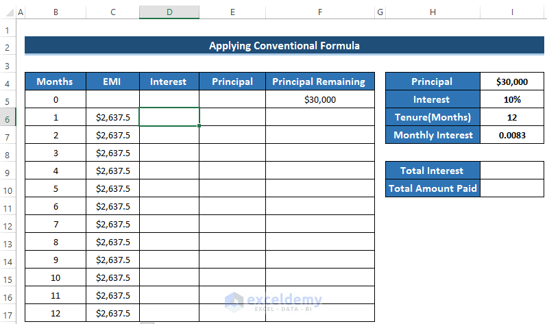
• Interest is equal to the product of monthly interest and the previous principal remaining.
• Enter the following formula.

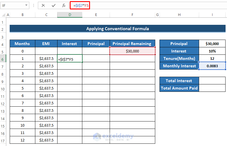
• Press Enter to apply the formula.

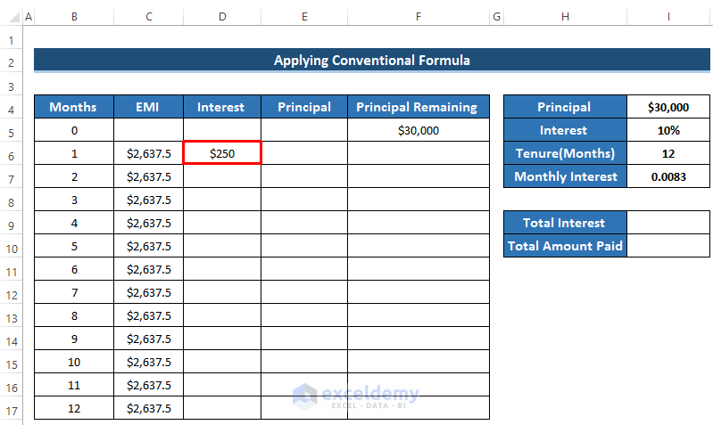
• This interest will go to the bank. We need to calculate the principal amount which can be subtracted from the principal loan amount.
• To calculate the principal, select cell E6.

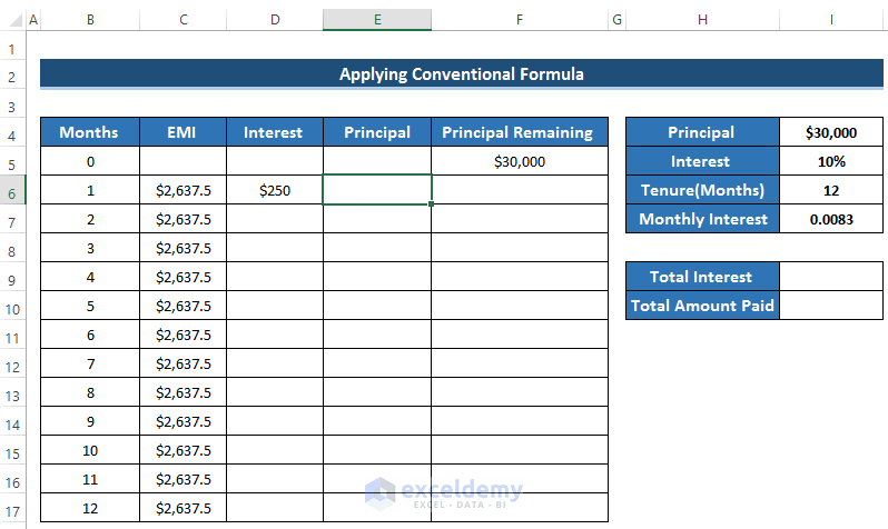
• The principal amount can be calculated by subtracting the interest value from EMI.
• Enter the following formula.

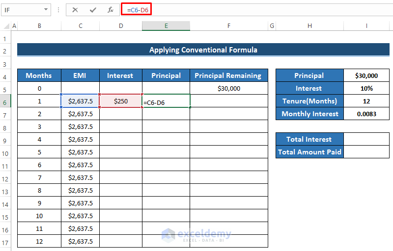
• Press Enter to apply the formula.

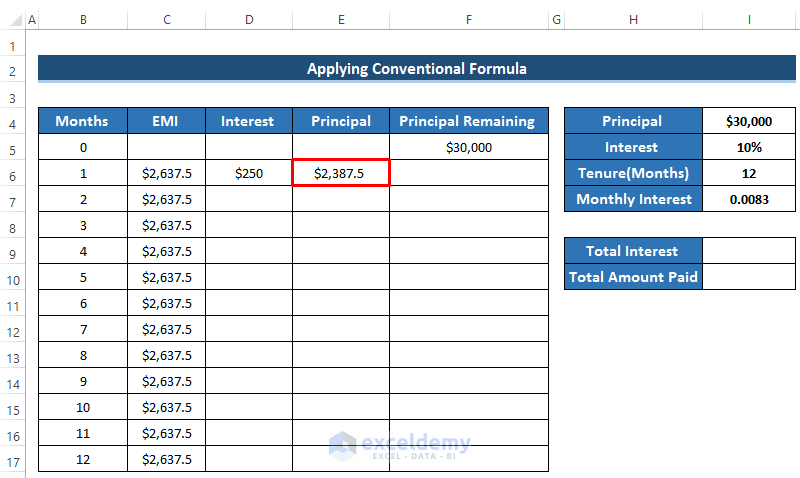
• Calculate the principal remaining.
• Select cell F6.

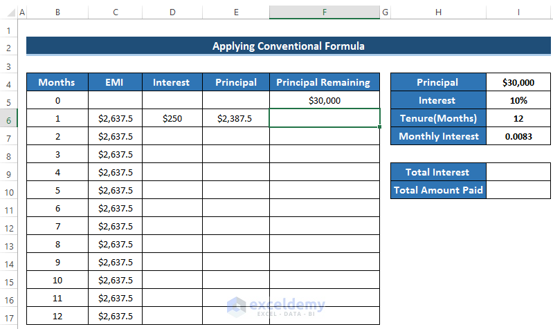
• To calculate the principal remaining, we need to subtract the principal value from the previous principal remaining value.
• The first principal remaining value is equal to the amount of loan you take.
• Enter the formula using the ABS function to avoid any negative value.

• Press Enter to apply the formula.

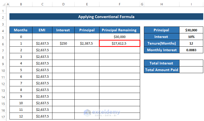
• After calculating the interest, EMI and principal, the interest and principal depend on the previous principal remaining.
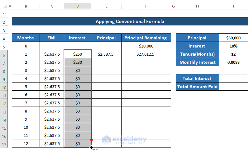
• Drag the Fill Handle icon of the interest column from D6 to D17.
• Some of the interest will be zero because it depends on the previous principal remaining. But in the 3rd month, the principal remaining cell is blank.

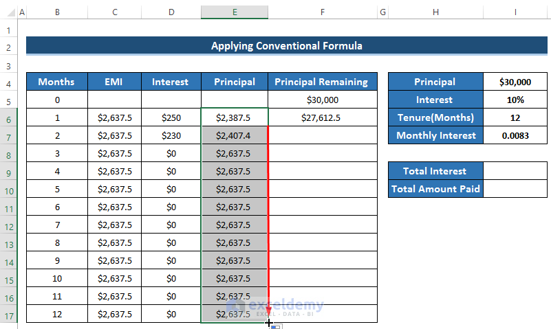
• Drag the Fill Handle icon of the principal column from cell E6 to E17.

• Drag the Fill Handle icon of the principal remaining column from F6 to F17.

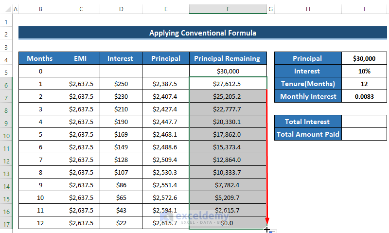
• You will see the change in the total dataset. Because when you have the previous principal remaining amount, the interest value can be calculated. By using the new interest the principal amount will be changed. This will happen in every cell until the principal remaining becomes zero.
• We get the desired result when the principal remaining becomes zero which means the loan is paid perfectly.

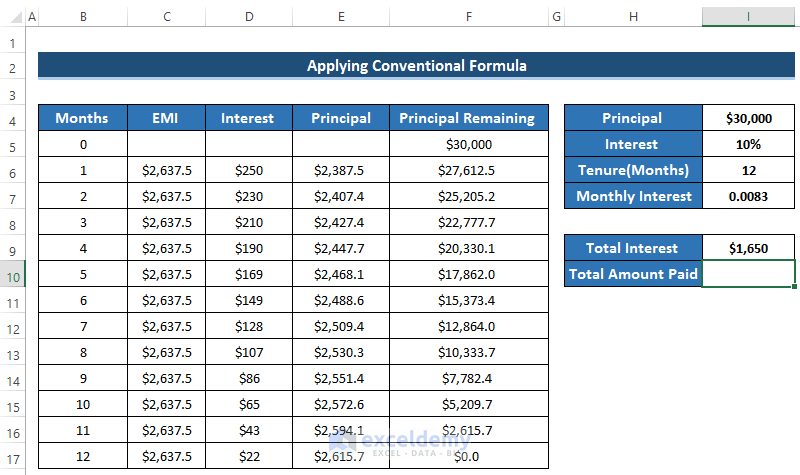
• To calculate the total interest, select cell I9.

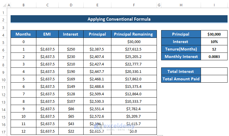
• Add all the interest paid in the 12 months using the SUM function.
• Enter the following formula.

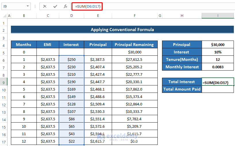
• Press Enter to apply the formula.

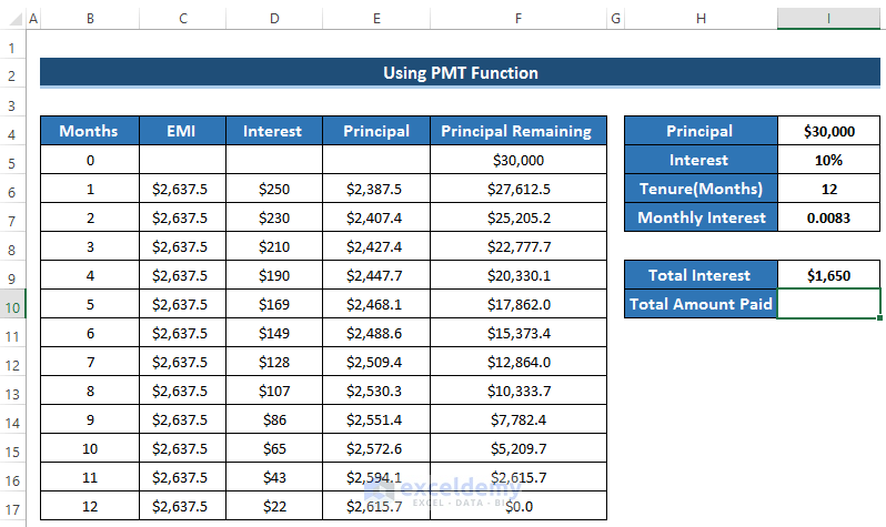
• To calculate the total amount paid which is the summation of total interest and principal, select cell I10.

• Enter the following formula to calculate the total amount paid using the SUM function.

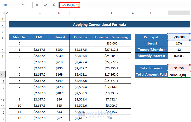
• Press Enter to apply the formula.
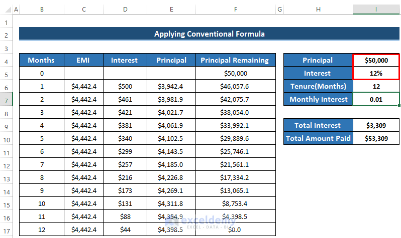
• We now have our final personal loan EMI calculator using the conventional method.

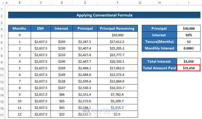
• If you change the principal and interest rate, the whole dataset will change according to it.
• If we take a principal loan of $5000 and an interest rate of 12%.
• We have the following output.

Read More: Home Loan EMI Calculator with Reducing Balance in Excel

Example 2 – Using PMT Function

Steps

• Select cell C7.

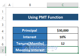
• The monthly interest is the ratio of the interest rate and the total monthly.
• Enter the following formula.

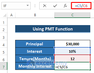
• Press Enter to apply the formula.

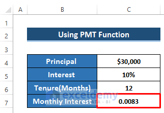
• Take this into a single worksheet where you would like to create the EMI.
• Create some row headers including EMI, interest, principal and principal remaining.
• The principal remaining is the total amount of loan that you take.
• After 12 months, the principal remaining must be zero.

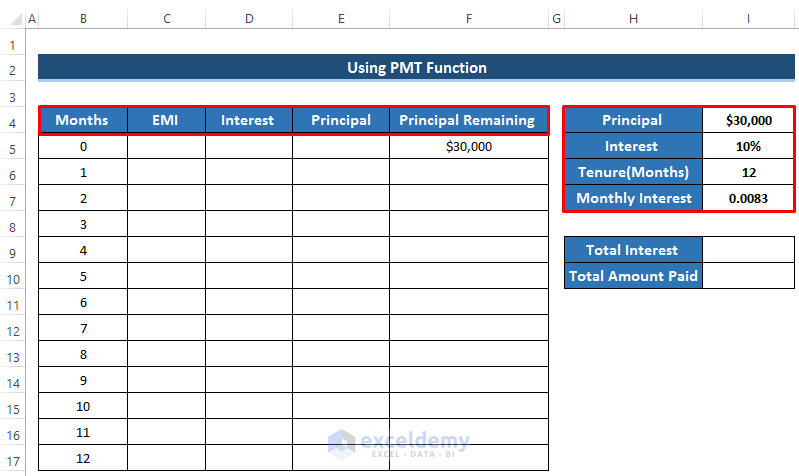
• To calculate the EMI in the first month, select cell C6.

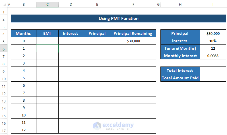
• To calculate the EMI, enter the formula using the ABS and PMT functions.

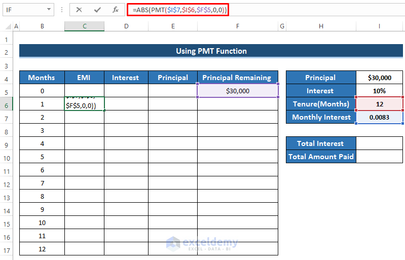
• Press Enter to apply the formula.

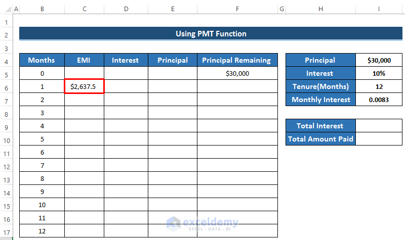
• You need to have the same EMI for every value. So, if you look at the formula, you will find all the cells are made constant by using the ($) sign.
• Drag the Fill Handle icon down the column up to cell C17. That is our EMI for that specific loan amount and the specific interest rate.

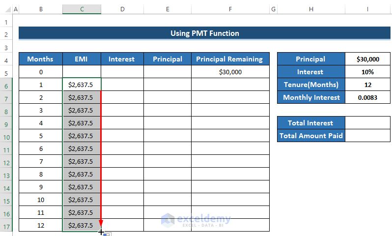
• Calculate the interest.
• Select cell D6.

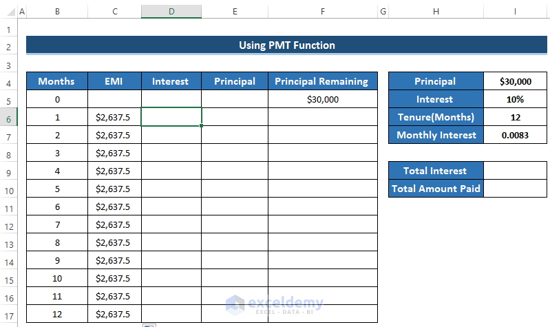
• Interest is equal to the product of monthly interest and the previous principal remaining.
• Enter the following formula

• Press Enter to apply the formula.

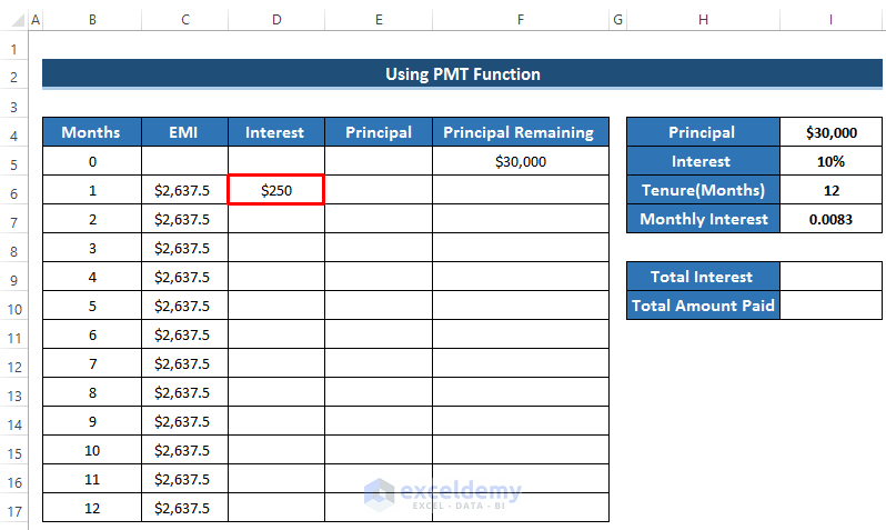
• This interest will go to the bank. We need to calculate the principal amount which can be subtracted from the principal loan amount.
• To calculate principal, select cell E6.

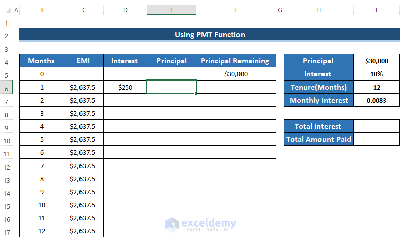
• The principal amount can be calculated by subtracting the interest value from EMI.
• Enter the following formula.

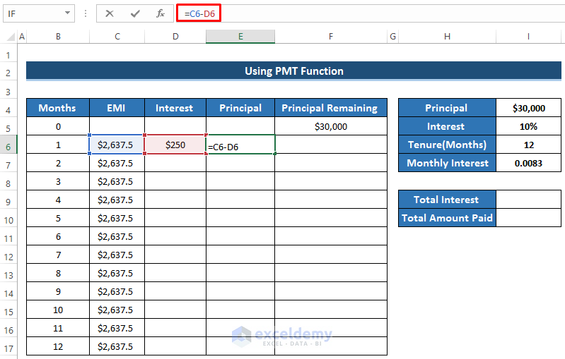
• Press Enter to apply the formula.

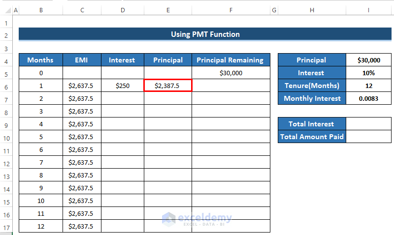
• Calculate the principal remaining.
• Select cell F6.

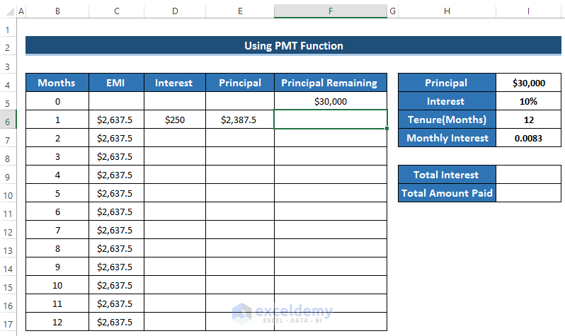
• To calculate the principal remaining, we need to subtract the principal value from the previous principal remaining value.
• The first principal remaining value is equal to the amount of loan you take.
• Enter the following formula.

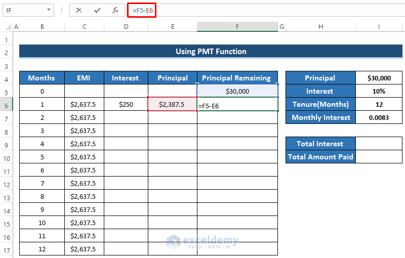
• Press Enter to apply the formula.

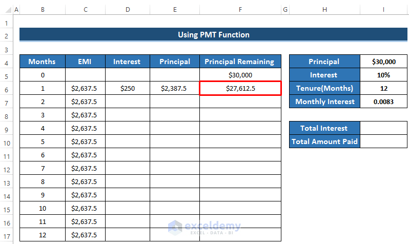
• After calculating the interest, EMI, and principal, the interest and principal depend on the previous principal remaining.
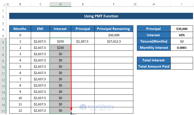
• Drag the Fill Handle icon of the interest column from D6 to D17.
• Some of the interest will be zero because it depends on the previous principal remaining. But in the 3rd month, the principal remaining cell is blank.

• Drag the Fill Handle icon of the principal column from cell E6 to E17.

• Drag the Fill Handle icon of the principal remaining column from F6 to F17.

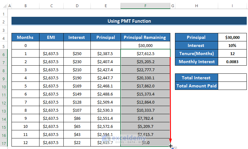
• You will see the change in the total dataset. Because when you have the previous principal remaining amount, the interest value can be calculated. By using the new interest the principal amount will be changed. This will happen in every cell until the principal remaining becomes zero.
• We get the desired result when the principal remaining becomes zero which means the loan is paid perfectly.

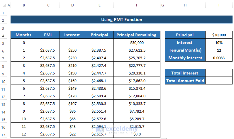
• To calculate the total interest, select cell I9.

• Enter the following formula.

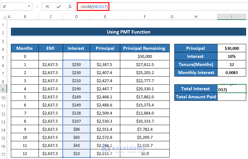
• Press Enter to apply the formula.

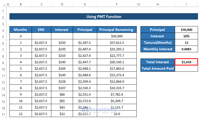
• To calculate the total amount paid which is the summation of total interest and principal, select cell I10.

• Enter the following formula to calculate the total amount paid using the SUM function.

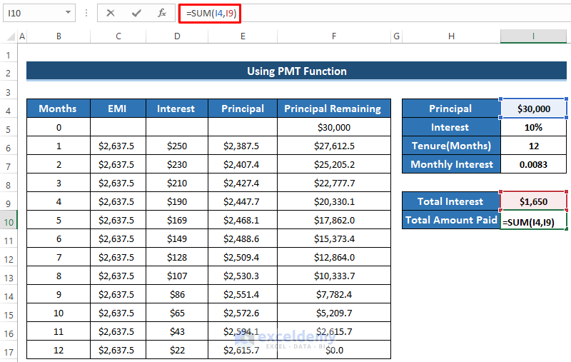
• Press Enter to apply the formula.

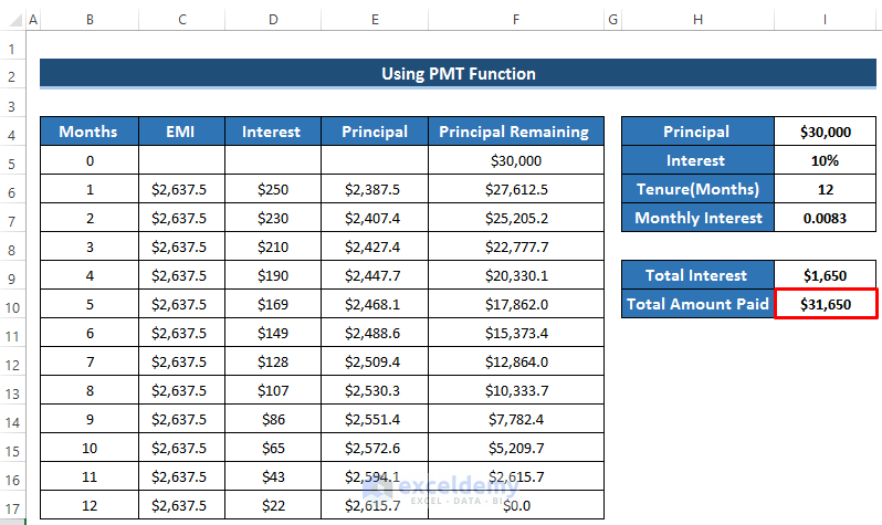
• You will get the personal loan EMI calculator using the PMT function.

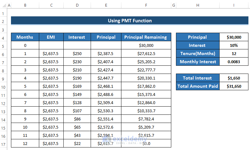
• If you change the principal and interest rate, the whole dataset will change according to it.
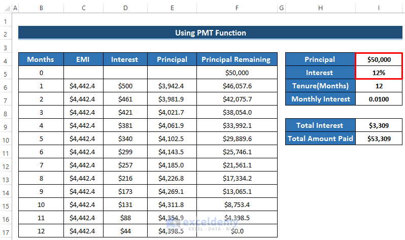
• If we take a principal loan of $5000 and an interest rate of 12%.
• We have the following output.

Read More: EMI Calculator with Prepayment Option in Excel Sheet

Things to Remember

• To calculate the principal remaining, we need to subtract the principal rather than EMI because we have to pay the interest to the bank. The principal amount is calculated by subtracting interest from EMI.
• While using the conventional method, you need to apply the bracket carefully. Otherwise, there will be a change in overall calculation.

Download Practice Workbook

Related Articles

• SBI Home Loan EMI Calculator in Excel Sheet with Prepayment Option
• Create Home Loan EMI Calculator in Excel Sheet with Prepayment Option
• Reducing Balance EMI Calculator in Excel Sheet
• How to Create Reverse EMI Calculator in Excel

<< Go Back to EMI Calculator | Finance Template | Excel Templates