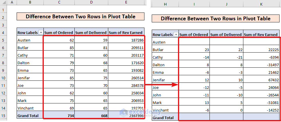
We have a dataset that contains information about several sales representatives of the Armani group. The names of the sales representatives and the sums of the ordered product, delivered product, and the revenue earned by the sales representatives are given in columns B, C, D, and E, respectively. We will calculate the difference between two rows in the Pivot Table.
Step 1 – Create a Pivot Table
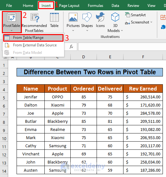
- Select any cell in the dataset.
- Go to Insert and select PivotTable, then choose From Table/Range.
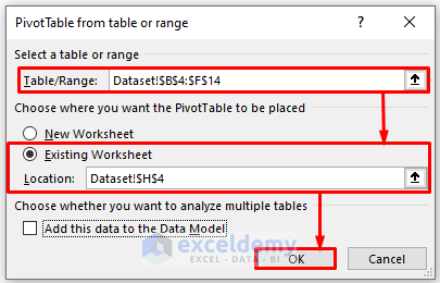
- A dialog box named PivotTable from table or range will appear.
- Insert the data range locations in the Table/Range box.
- Select Existing Worksheet under Choose where you want the PivotTable to be placed.
- Press OK.
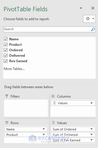
- Add (by dragging) Name and Product to the Rows area, Values to the Columns area, and Ordered, Delivered, and Rev Earned to the Values area.
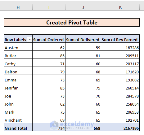
- Here’s the resulting pivot table from our sample dataset.
Read More: Excel Pivot Table: Difference between Two Columns
Step 2 – Calculate the Differences Between Two Rows in a Pivot Table
- Select any cell in the Pivot Table. We chose cell I5.
- Right-click on the cell and select Show Values As.
- Select the Difference From option.
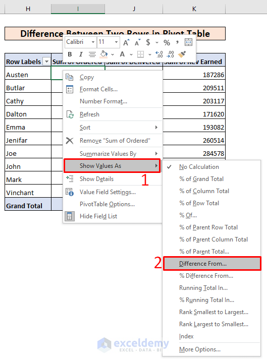
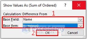
- A dialog box named Show Values As ( Sum of Order)? will appear.
- Select Name from the drop-down box for Base Field.
- Select (previous) from the drop-down box for Base Item. We selected (previous) because we want to calculate the difference from the second row to first row.
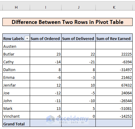
- You will calculate the difference between two rows in the Pivot Table which has been given in the below screenshot.
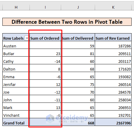
- Calculate the difference for the rest of the columns between two rows in the Pivot Table in a similar manner.
Read More: Pivot Table: Percentage Difference between Two Columns
Things to Remember
- While a value can’t be found in the referenced cell, the #N/A error appears in Excel.
Download the Practice Workbook
<< Go Back to Difference in Pivot Table | Pivot Table in Excel | Learn Excel
Get FREE Advanced Excel Exercises with Solutions!

