Step 1 – Create Basic Outlines
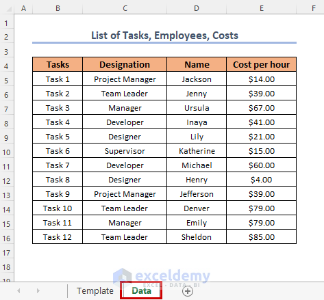
- In the Data sheet, enter the tasks, employee names, their designation, and costs per hour to complete each task.
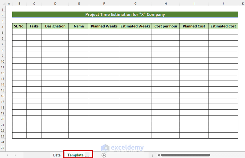
- Create another sheet: Template.
- Insert 7 columns; SL No, Tasks, Designation, Name, Planned Weeks; Estimated Weeks, Cost per hour, Planned Cost, and Estimated Cost.
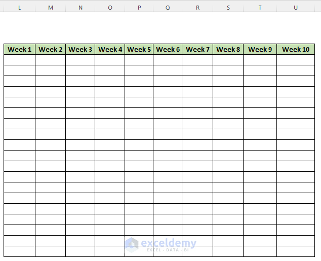
- Add 10 more columns for 10 weeks to see the percentage of accomplished tasks.
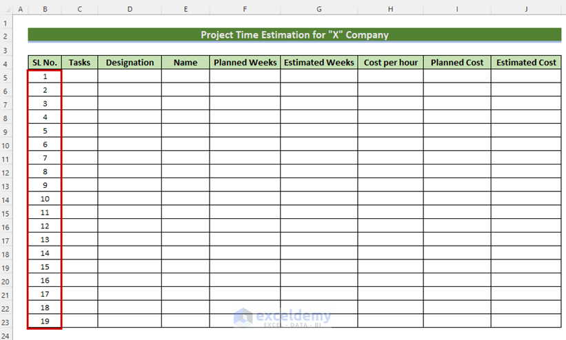
- Add serial numbers from 1 to 19 in SL No.
Read More: How to Calculate Residential Construction Cost Estimator in Excel
Step 2 – Create a Drop-down List and Enter Values
- Select the Tasks column and go to the Data tab >> Data Validation.
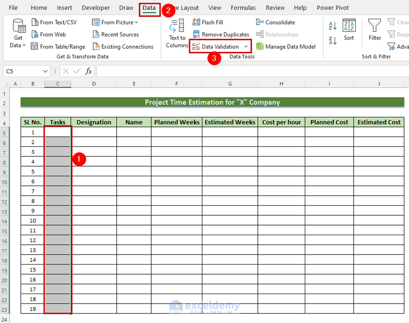
In the Data Validation dialog box:
- Select the List in Allow.
- Choose the list of Tasks in the Data sheet and click OK.
- The following formula is displayed in the Source box.
=Data!$B$5:$B$16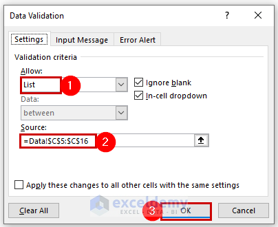
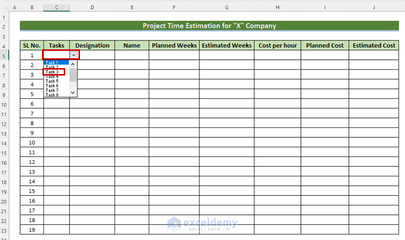
You will see the symbol of the drop-down list in the Tasks column.
- Click the drop-down sign in C5 and choose a task from the list. Here, Task 3.
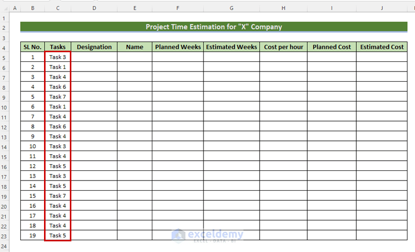
- Complete the other cells in the Tasks column by choosing different tasks from the list.
- Select the cells in the Designation column and go to the Data tab >> Data Validation.
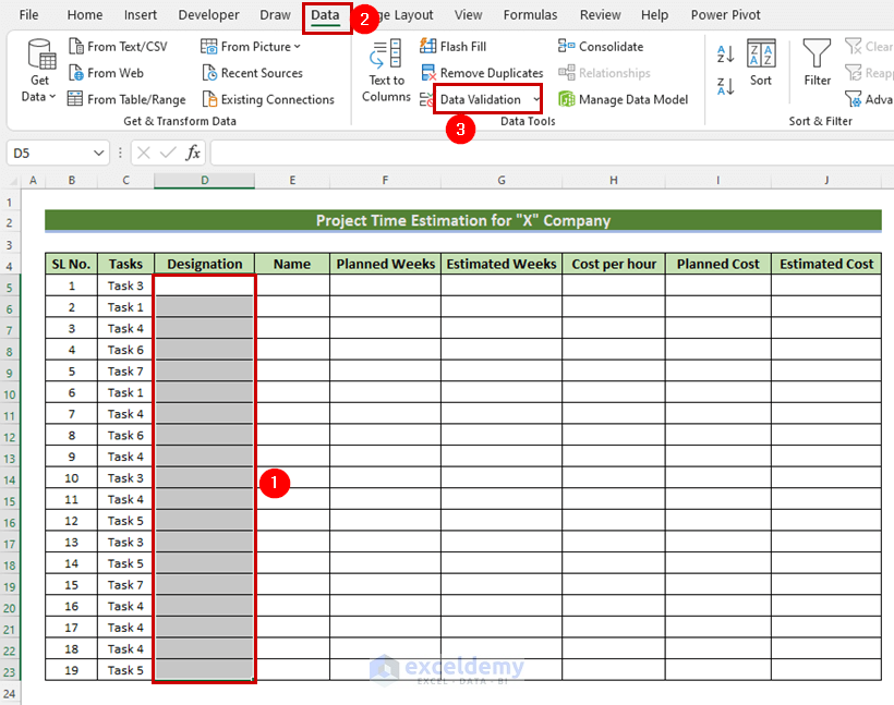
In the Data Validation dialog box:
- Select List in Allow.
- Select the column Designations in the Data sheet.
- Click OK.
- The following formula will be displayed in the Source box.
=Data!$C$5:$C$16
The drop-down list symbol is displayed in the Designation column.
- Click the drop-down sign inD5 and choose a Designation. Here, Manager.
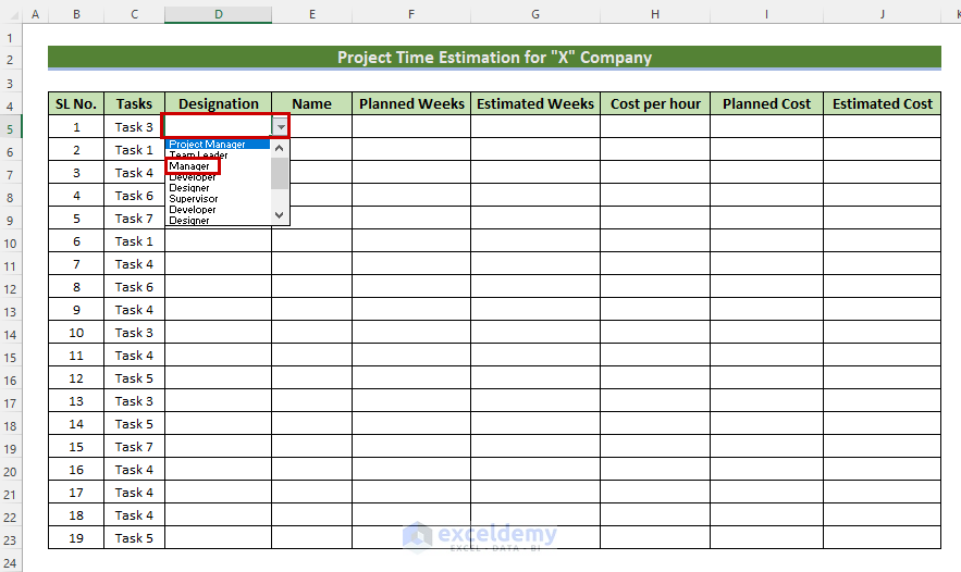
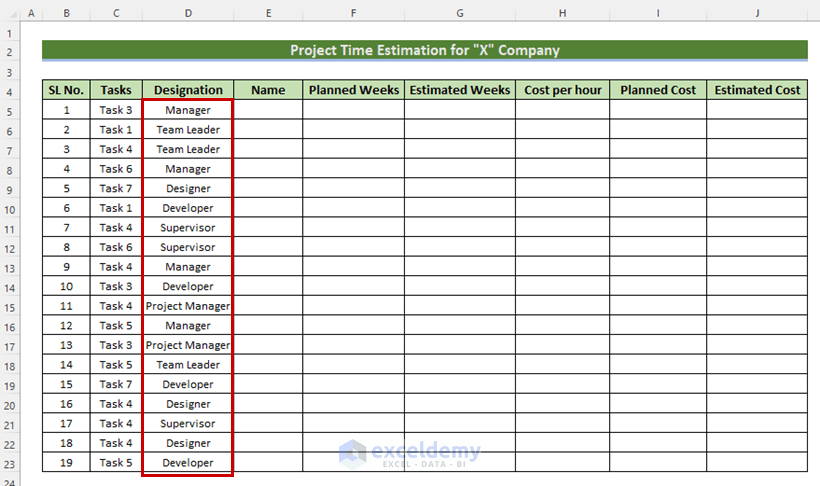
Complete the other cells in the Designation column by choosing different designations from the list.
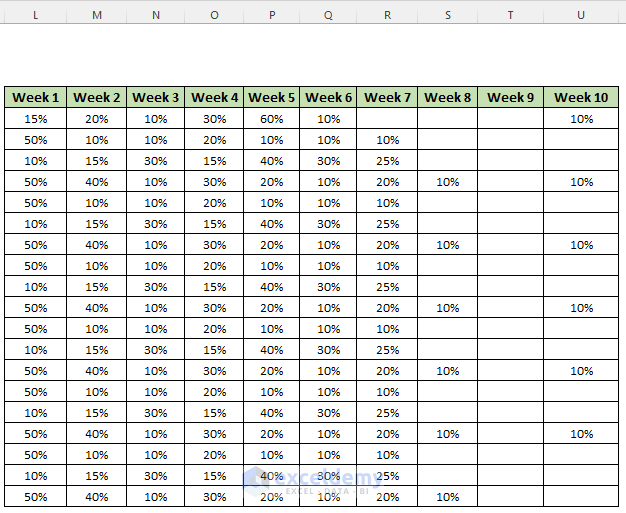
- Enter the percentages of tasks completed in different weeks:
Read More: How to Make an Effort Estimation Sheet in Excel
Step 3 – Applying Formulas
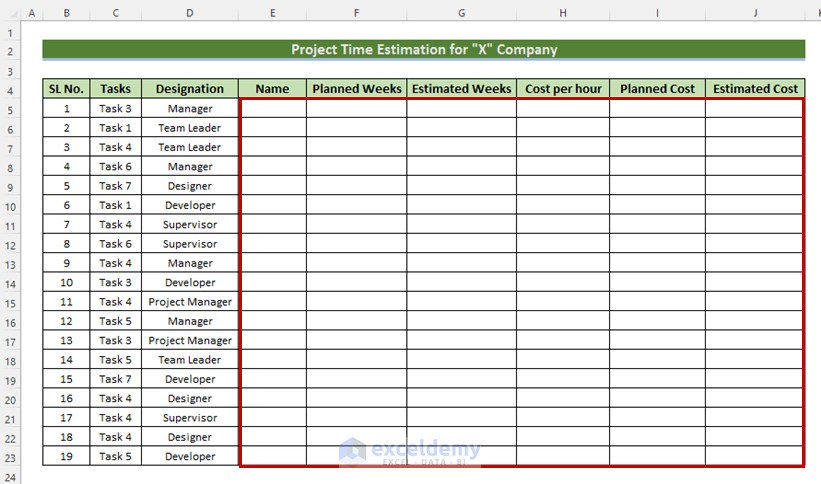
- Use the following formula in E5 to get the names corresponding to different designations.
=INDEX(Data!$D$5:$D$16, MATCH(D5, Data!$C$5:$C$16,0))Formula Breakdown
- MATCH(D5, Data!$C$5:$C$16,0) → becomes
- MATCH(“Manager”, Data!$C$5:$C$16,0) → The MATCH function returns the row index number corresponding to $C$5:$C$16: Manager
- Output → 3
- MATCH(“Manager”, Data!$C$5:$C$16,0) → The MATCH function returns the row index number corresponding to $C$5:$C$16: Manager
- INDEX(Data!$D$5:$D$16, MATCH(D5, Data!$C$5:$C$16,0)) → becomes
- INDEX(Data!$D$5:$D$16, 3) → The INDEX function returns the name of the employee in Row 3 in $D$5:$D$16.
- Output → Ursula
- INDEX(Data!$D$5:$D$16, 3) → The INDEX function returns the name of the employee in Row 3 in $D$5:$D$16.
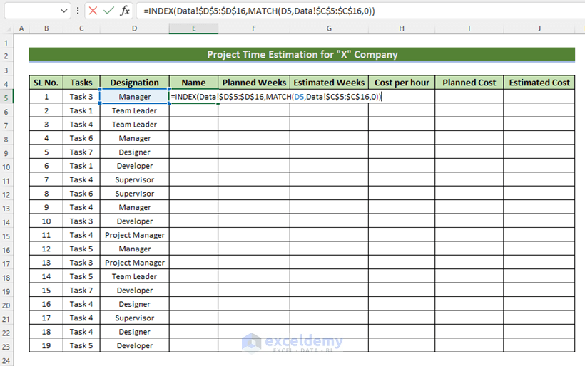
- Press ENTER and drag down the Fill Handle.
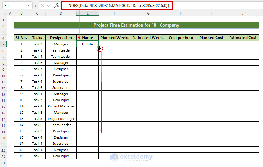
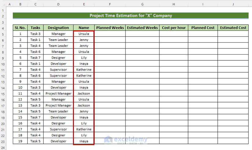
You will see the employees’ names and their designations.
To extract the costs of different tasks from the Data sheet.
- Enter the following formula in H5 and press ENTER.
=INDEX(Data!$E$5:$E$16, MATCH(C5, Data!$B$5:$B$16,0))Formula Breakdown
- MATCH(C5, Data!$B$5:$B$16,0) → becomes
- MATCH(“Task 3”, Data!$B$5:$B$16,0) → The MATCH function returns the row index number corresponding to $C$5:$C$16: Manager
- Output → 3
- MATCH(“Task 3”, Data!$B$5:$B$16,0) → The MATCH function returns the row index number corresponding to $C$5:$C$16: Manager
- INDEX(Data!$E$5:$E$16, MATCH(C5, Data!$B$5:$B$16,0)) → becomes
- INDEX(Data!$E$5:$E$16, 3) → The INDEX function returns the cost of the corresponding task in Row 3 in $E$5:$E$16.
- Output → $67.00
- INDEX(Data!$E$5:$E$16, 3) → The INDEX function returns the cost of the corresponding task in Row 3 in $E$5:$E$16.
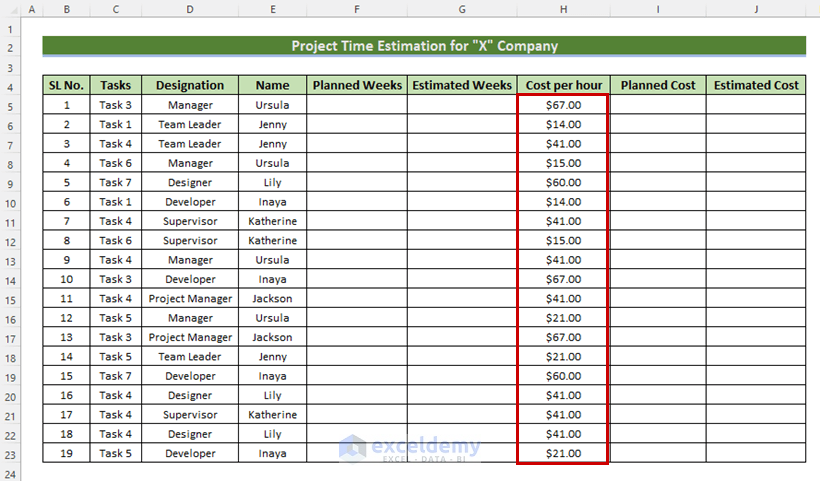
- Drag down the Fill Handle.
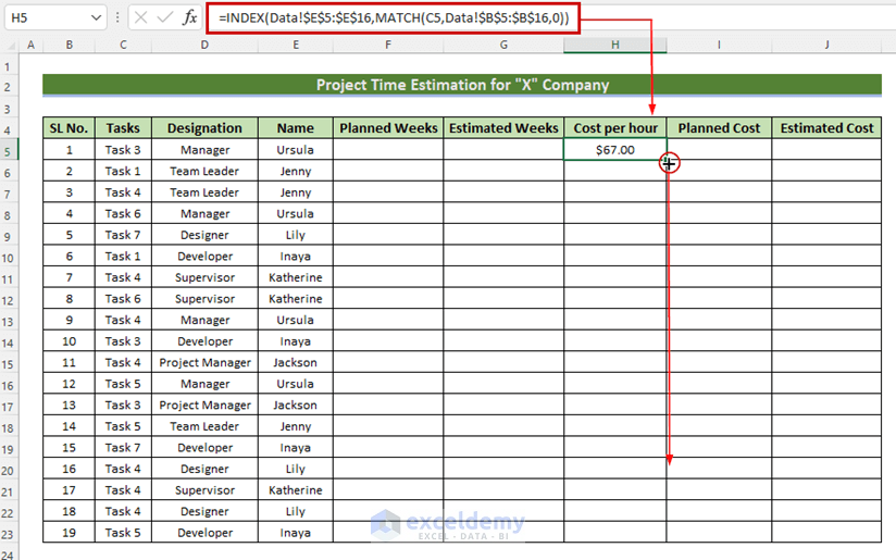
The costs of different tasks are displayed.
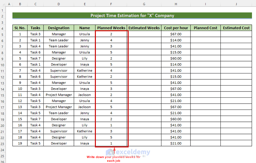
- Enter the planned number of weeks for different tasks in the Planned Weeks column.
To calculate the time for completing each task based on the percentages of different tasks in different weeks:
- Use the following formula in G5 and press ENTER.
=IF(SUMIF($L5:$U5,">0")>0, SUMIF($L5:$U5,">0"),"")Formula Breakdown
- SUMIF($L5:$U5,”>0″) → The SUMIF function sums the percentages in $L5:$U5 if values are greater than 0.
- Output → 1.55
- IF(SUMIF($L5:$U5,”>0″)>0, SUMIF($L5:$U5,”>0″),””) → becomes
- IF(1.55>0, 1.55,””) → The IF function returns 55: the logical condition is TRUE. Otherwise, blank.
- Output → 1.55
- IF(1.55>0, 1.55,””) → The IF function returns 55: the logical condition is TRUE. Otherwise, blank.
- Drag down the Fill Handle.
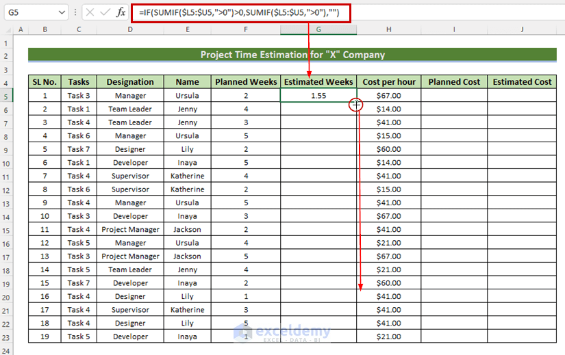
The estimated weeks for different tasks are displayed.
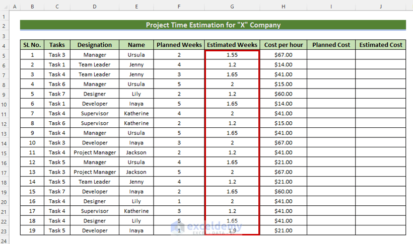
To calculate the costs of the planned duration:
- Use the following formula in I5 and press ENTER.
=IF(H5<>"",$F5*H5*5*8,"")Formula Breakdown
- $F5*H5*5*8 → becomes
- 2*67*5*8 → multiplies the total weeks by cost per hour; to convert the total weeks into hours, weeks are multiplied by 5 (weekdays) and 8 (daily working hours).
- Output → 5360
- 2*67*5*8 → multiplies the total weeks by cost per hour; to convert the total weeks into hours, weeks are multiplied by 5 (weekdays) and 8 (daily working hours).
- IF(H5<>””,$F5*H5*5*8,””) → becomes
- IF(67<>””,5360,””) → returns 5360: the logical condition is TRUE. Otherwise, blank.
- Output → 5360
- IF(67<>””,5360,””) → returns 5360: the logical condition is TRUE. Otherwise, blank.
- Drag down the Fill Handle.
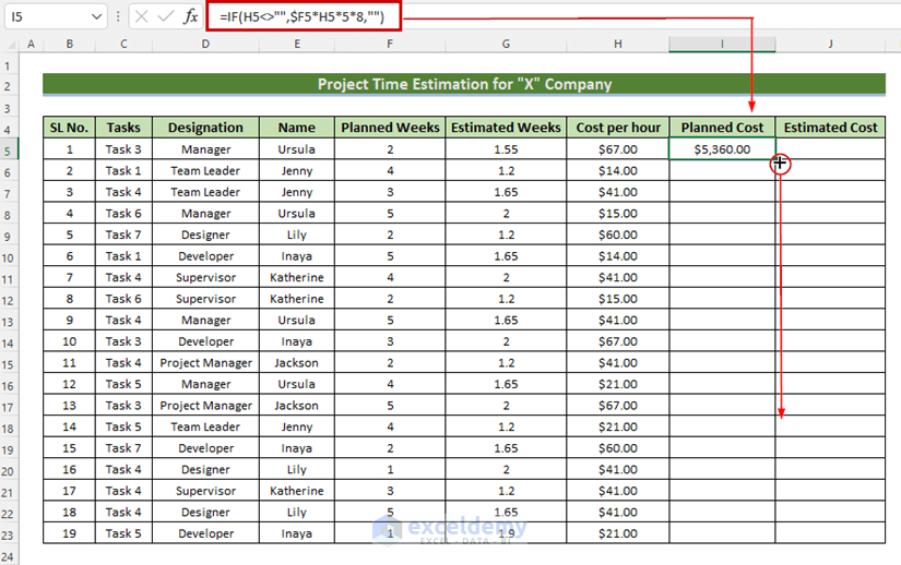
The costs of each task according to the planned data are displayed:
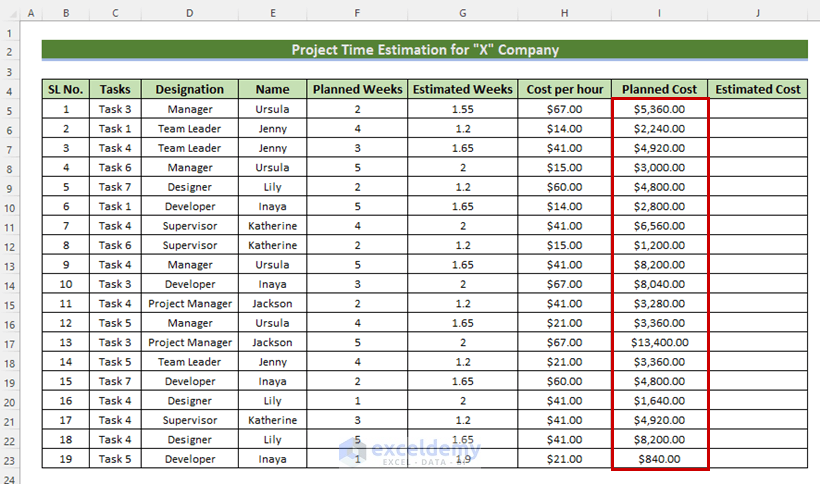
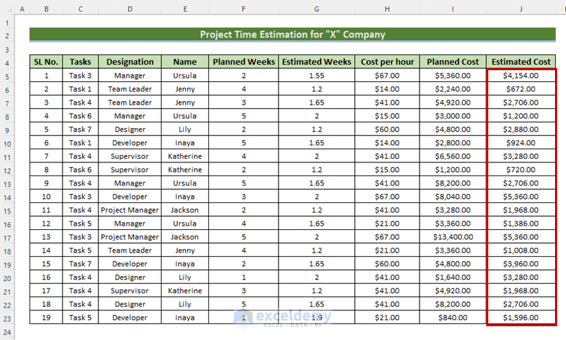
- Enter the following formula in J5 and press ENTER.
=IF(H5<>"",$G5*H5*5*8,"")Formula Breakdown
- $G5*H5*5*8 → becomes
- 55*67*5*8 → multiplies the total weeks by cost per hour; to convert the total weeks into hours, they are multiplied by 5 (weekdays) and 8 (daily working hours).
- Output → 4154
- 55*67*5*8 → multiplies the total weeks by cost per hour; to convert the total weeks into hours, they are multiplied by 5 (weekdays) and 8 (daily working hours).
- IF(H5<>””,$G5*H5*5*8,””) → becomes
- IF(67<>””,4154,””) → returns 4154: the logical condition is TRUE. Otherwise, blank.
- Output → 4154
- IF(67<>””,4154,””) → returns 4154: the logical condition is TRUE. Otherwise, blank.
- Drag down the Fill Handle.
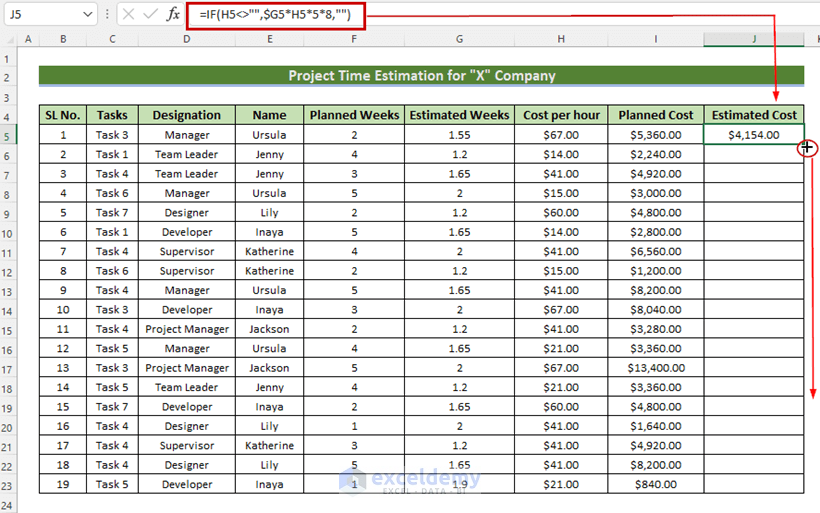
The costs of each task are displayed.
Read More: How to Make Cost Estimation Sheet in Excel
Step 4 – Calculating the Total Values
Calculate the total weeks and total costs of all projects:
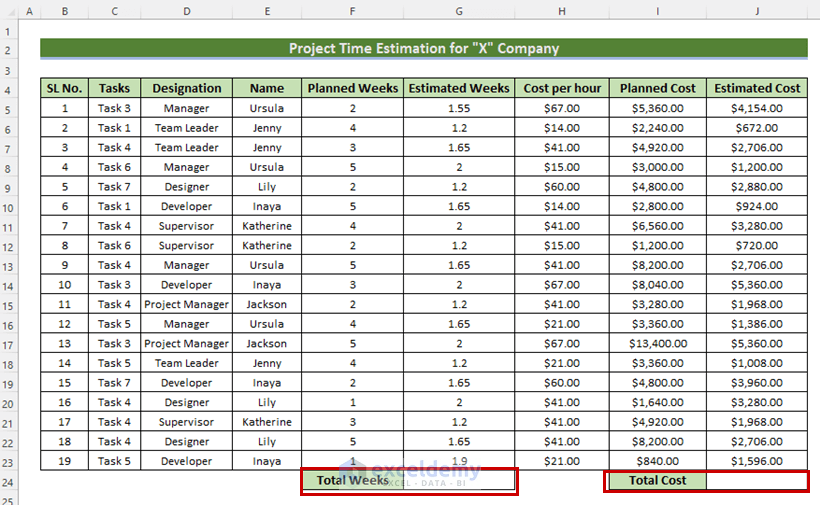
- Enter the following formula in G24.
=SUM(G5:G23)The SUM function returns the total number of weeks.
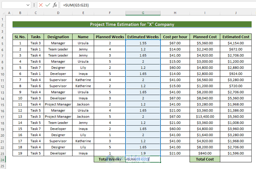
- Press ENTER.
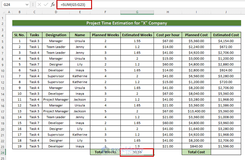
Calculate the number of weeks required to complete all tasks:
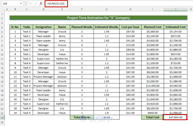
- Enter the following formula in J24.
=SUM(J5:J23)The SUM function returns the total costs of all tasks.
Download Practice Workbook
Related Articles
- How to Do Interior Estimation in Excel
- Project Cost Estimation Example in Excel
- How to Make House Estimate Format in Excel
<< Go Back to Excel Project Management Templates | Excel Templates
Get FREE Advanced Excel Exercises with Solutions!

