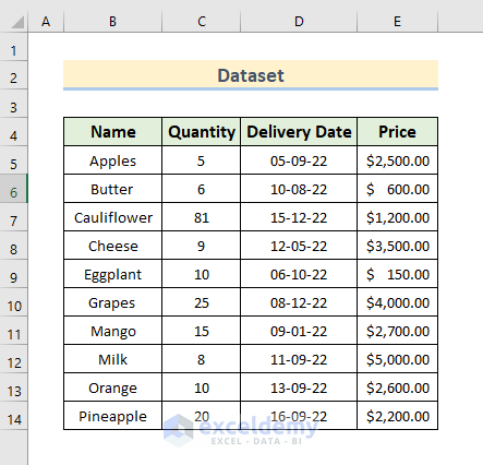
How to Perform Random Sort in Excel (6 Easy Methods)

We will show 6 easy methods to random sort in Excel, using a dataset of a shop containing product Name, Quantity, Delivery Date, and Price.

Method 1 – Use the RAND Function to Perform a Random Sort in Excel

The RAND function generates a random fractional number between 0 and 1.

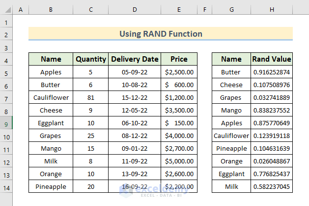
Make two additional columns Name and Rand Value outside of the main dataset (columns G and H) and copy the names from the Name column.
Insert the following formula in Cell H5.

=RAND()

Press Enter.

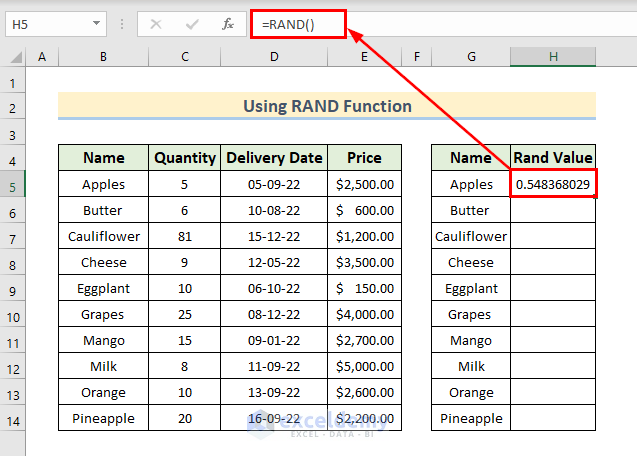
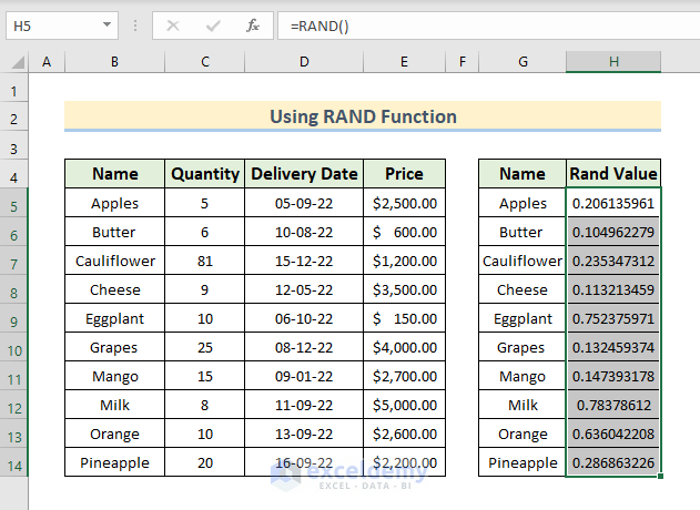
The value returned is greater than or equal to 0 and less than 1.

Use the Fill Handle to copy the formula to the cells below.

Select the random values in the Rand Value column.

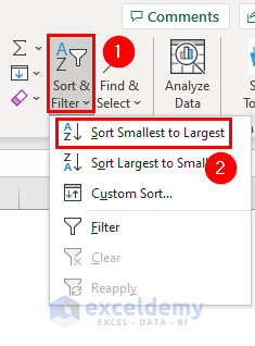
Select Sort & Filter then choose Sort Smallest to Largest in the Home tab of Excel

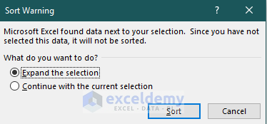
A Sort Warning window will appear.
Select Expand the section and press Sort.

The values from the new Name column are sorted randomly.

Read More: How to Sort Drop Down in Excel

Method 2 – Perform a Random Sort with the RAND Function while Keeping the List Order

Add an extra column Sort Order.
In the Sort Order, column generate random values using the RAND function like in Method 1.

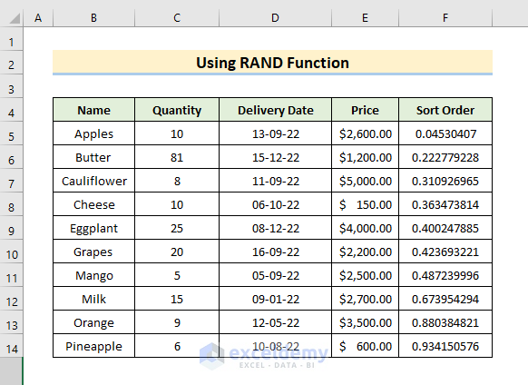
Select data from the Sort Order column and select Sort & Filter, then choose Filter in the Home tab.

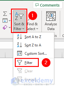
The filter icon will appear in the Sort Order column.
Click on the drop-down icon and select Sort Smallest to Largest from the options.

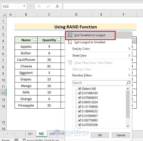
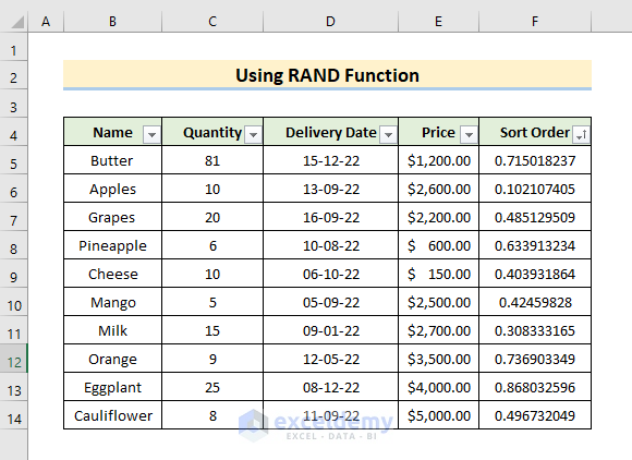
The dataset will be sorted randomly.

Method 3 – Use Excel RAND and SORT Functions to Do a Random Sort

We’ll use the same dataset.

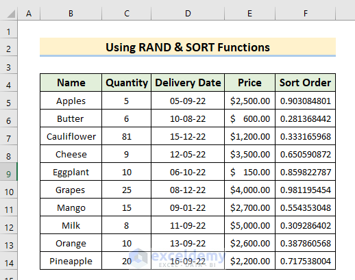
Add a sort number column and insert random values in it.
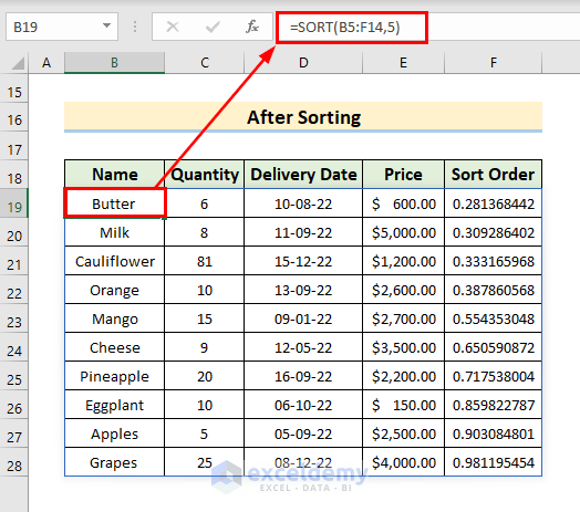
Create another table without data in it.
Use the following formula in Cell B19.

=SORT(B5:F14,5)

Press Enter.

5:F14 is the range where our data is present. 5 is used as we have six columns.

Note: we used an array formula. For versions of Excel except Excel 365, press Ctrl + Shift + Enter instead of pressing only Enter.

Method 4 – Insert SORTBY, RANDARRAY, and ROWS Functions to Do a Random Sort

We’ll start with the dataset with the added Sort Order column populated by random numbers.

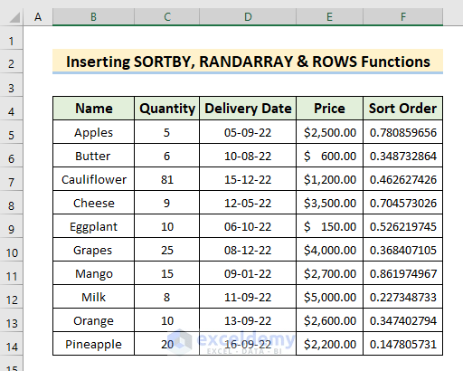
Create another table without data in it.
Use the following formula in Cell B19.

=SORTBY(B5:F14,RANDARRAY(ROWS(B5:B14)))

Press Enter.

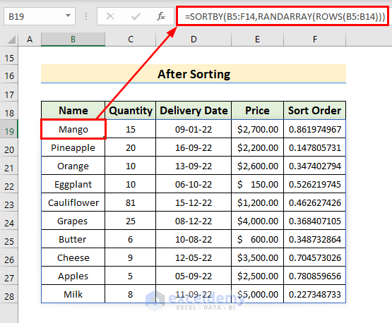
In the SORTBY function, B5:F14 is the range where the sorting will be performed.
The second argument of the SORTBY function is by_array1. We have passed a random array by using the RANDARRAY. As we are generating random values for each row, we need to assign them using the ROWS function in each row.
The ROWS function here counts the total number of rows of the dataset from B5 to B14.

Method 5 – Utilize SORTBY, RANDARRAY, and COUNTA Functions for Random Sorting

We’ll use the same dataset.

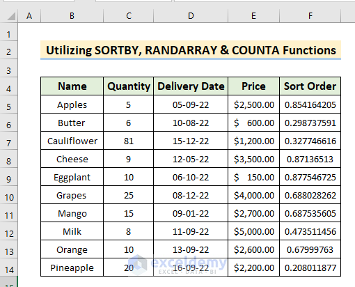
Copy the headers into the range B18:F18.
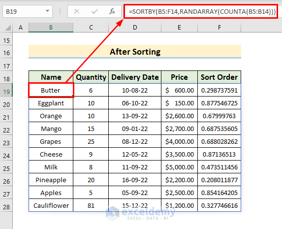
Use the following formula in Cell B19.

=SORTBY(B5:F14,RANDARRAY(COUNTA(B5:B14)))

Press Enter.

This formula is similar to the previous formula. Instead of using the ROWS function, we are using the COUNTA function which is doing the same thing by counting the row numbers.

Method 6 – Apply VBA for Random Sorting in Excel

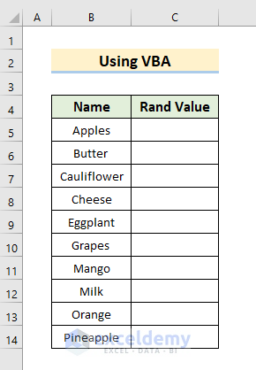
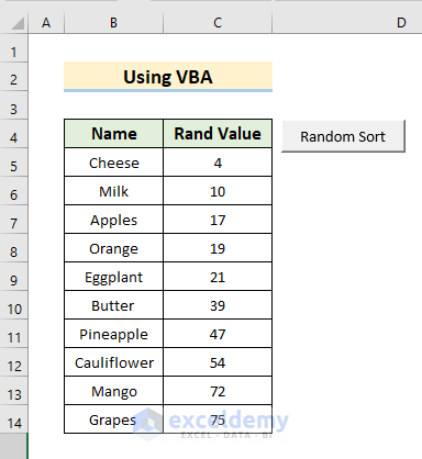
We have included a simple dataset with the columns Name and Rand Value.

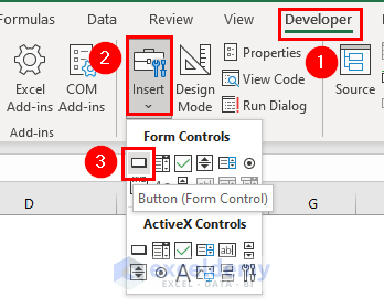
Go to the Developer tab and select Insert, then choose Button (Form Control).

A button will appear. Place the button in your worksheet.
Change the button name to Random Sort.
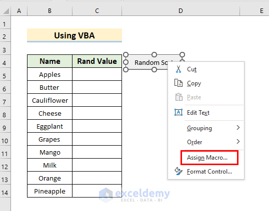
Right-click on the button and select Assign Macro.

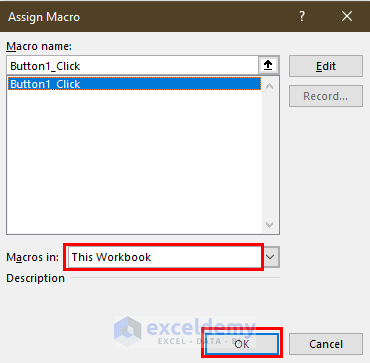
In the Assign Macro window, select This Workbook from Macros in section and press OK.

A VBA window will appear.
Insert the following code there.

Sub Random_Sort()
  Dim xtmpStr As String, xtmpInt As Integer, m As Integer, n As Integer
  For Z = 5 To 14
    Cells(Z, 3).Value = WorksheetFunction.RandBetween(0, 100)
 Next Z
  For m = 5 To 14
    For n = m + 1 To 14
  If Cells(n, 3).Value < Cells(m, 3).Value Then
  xtmpStr = Cells(m, 2).Value
  Cells(m, 2).Value = Cells(n, 2).Value
  Cells(n, 2).Value = xtmpStr
  xtmpInt = Cells(m, 3).Value
  Cells(m, 3).Value = Cells(n, 3).Value
  Cells(n, 3).Value = xtmpInt
  End If
      Next n
  Next m
End Sub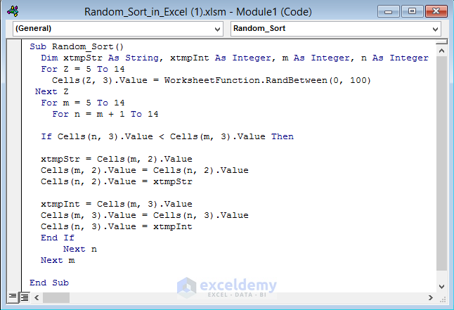

Save the VBA code by pressing Ctrl + S.
Go back to the worksheet and click on the Random Sort button.

Read More: Advanced Sorting in Excel

Things to Remember

Common Errors	When they show
#VALUE	If there is any blank cell in the dataset and if you use the SORTBY function on that dataset this error will occur.
#SPILL	As with any other dynamic array function, a #SPILL! The error most often means that there isn’t enough space in the intended spill range to display all the results.
#NAME	If the function’s name is misspelled, then this error will appear.