How to Rearrange Columns in Excel to Match Another Sheet (4 Ways)

Whenever you are working with a workbook in Excel that contains multiple sheets, It is important to rearrange one sheet so that it matches another sheet in that workbook. In addition, by rearranging the columns properly you can make it easier to find and read specific data. In this article, I am going to cover 4 simple ways on how to rearrange columns in Excel to match another sheet.

Why Do We Need to Rearrange Columns in Excel to Match Another Sheet?

• Rearranging columns in Excel to match another sheet is important when you are working on grouped worksheets.
• The arrangement of columns in an Excel worksheet is an important factor in its readability.
• Nevertheless, it is less time-consuming than entering data manually into a column to change the order.

Read More: How to Automatically Rearrange Columns in Excel

How to Rearrange Columns in Excel to Match Another Sheet: 4 Simple Ways

Here I have taken an Excel workbook that contains multiple worksheets that contain the same dataset with different arrangements. The dataset contains the Names of students and their Percentage Number of different subjects.

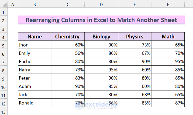
1. Using SHIFT and Drag to Rearrange Column to Match Another Sheet

Using the SHIFT key to drag and drop a column to rearrange the columns is the easiest way of rearranging columns. In this method, you can drag a column wherever you want. For this method, I want to match the order of the columns from the sheet named “Drag & Drop Command” to the sheet named “Dataset”

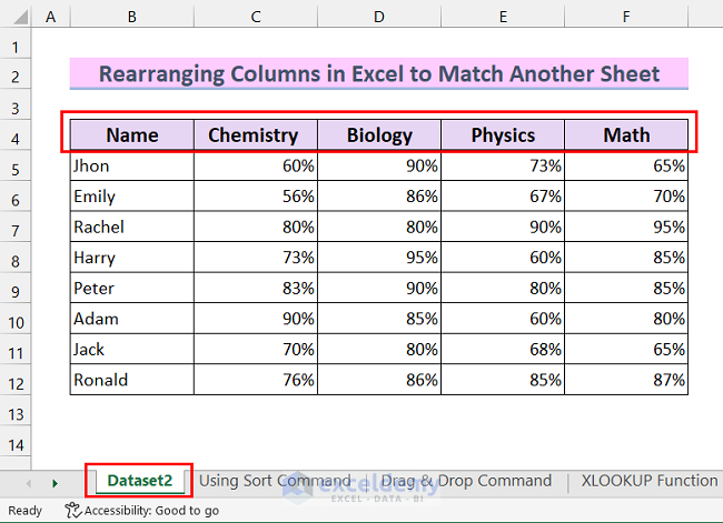
Let me show you the steps on how to rearrange columns in Excel to match another sheet by using the SHIFT key to drag the column across the sheet.

But remember to keep the dataset in the first row or avoid merging.

Steps:

• Firstly, select the column you want to move. Here, I have selected the column named
• Secondly, hold the SHIFT key and then drag the left or right border of the column.
• After that, drop the column in the position you want. Here, I have dropped the column after the column named Name.

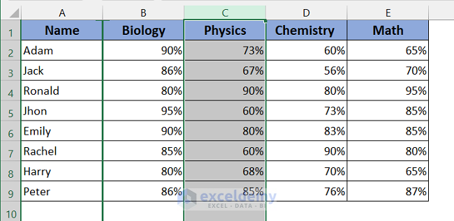
• Now, you can see that I have moved the Physics column successfully according to the order I want.

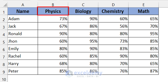
• After that, I followed the same steps to move the column Chemistry according to the order I want.

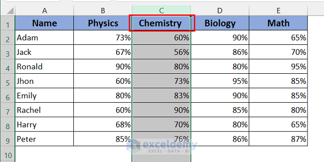
• And Finally, I have moved the column Biology to Column F and got my desired order as in sheet “Dataset”.

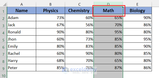
Here, you will get the rearranged column matches to another sheet.

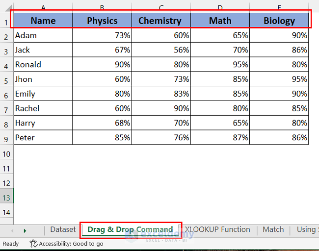
It should be noted that, while you are using this method there can not be any merged column over the table. If there are any merged columns over the table it will show an error and will not be able to perform the task successfully.

2. Use of Sort Command to Rearrange Column

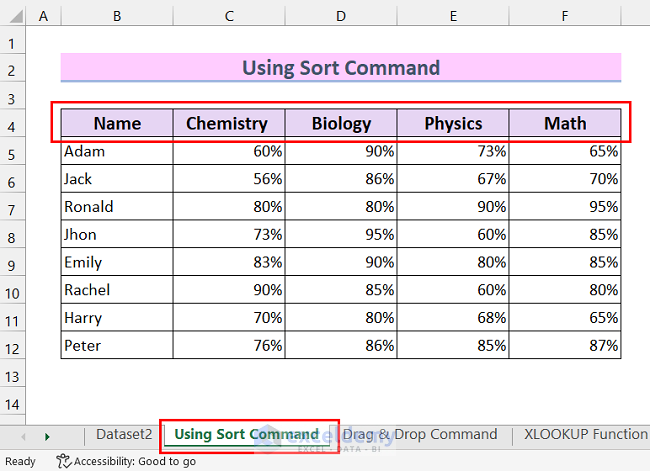
In this section, you will learn how to rearrange columns in Excel to match another sheet by the use of Data Sort. In this method, you will be able to sort all the columns at the same time, unlike the previous method. Here, I am matching the order of columns from sheet “Using Sort Command” to the order of the columns of sheet “Dataset2”

Let’s see step by step, how you can use data sort to rearrange columns in Excel to match another sheet.

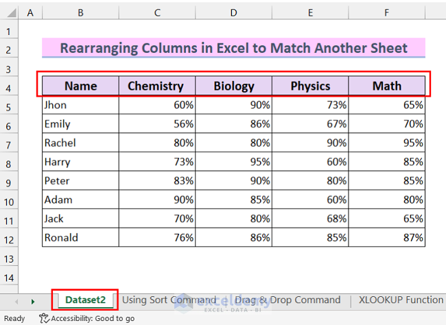
Steps:

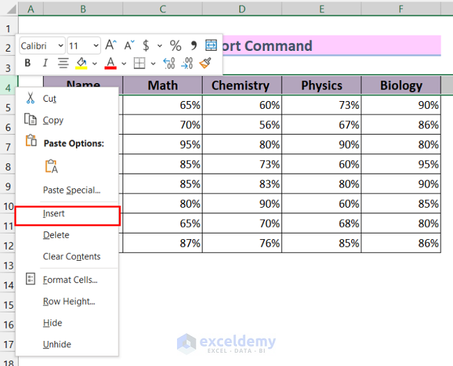
• To use data sort you at first have to insert a new row above the table. For that, you will have to right-click on the first row and then select Insert from the Context Menu. That will insert a new row at the top.

• In that new row, you will have to insert the new sorting order from your desired sheet. Here, I have inserted the sorting order according to the order of the sheet “Dataset2”

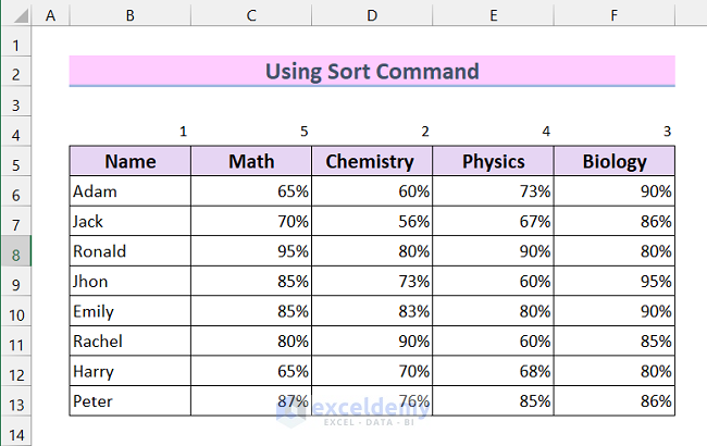
• Now, you will have to select the entire data table. Here, we selected the cell range B4:F13.
• Next, you will have to go to the Data menu and then select Sort from Sort and Filter.

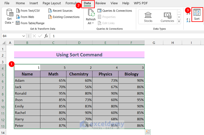
• Now, you will see that the Sort Dialog box will open up.
• Next, click Options and mark on Sort left to right and select Ok

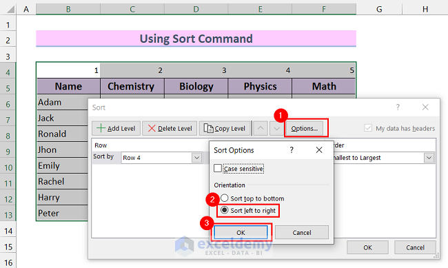
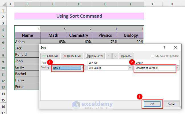
• And then, back in the Sort dialog box select the row in which you have inserted the sorting order in the Sort by menu. Here I have selected Row 4.
• After that select Smallest to Largest in the order field.
• Finally, select OK. That will sort your columns according to the order.

• Now, you can select the Entire first row you inserted at the beginning then Delete That will give you the exact table you want.

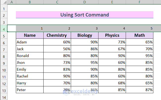
Here, You can see that the column order of my “Using Sort Command” sheet matches exactly with the “Dataset2” sheet.

3. Using XLOOKUP Function to Rearrange Columns to Match Another Sheet

You can use the XLOOKUP function to rearrange columns to match another sheet. In fact, it is a great way of rearranging columns according to a desired new order. And by using this formula you can get a new sorted table instead of changing the old one. Here, I used the nested XLOOKUP function to rearrange the column.

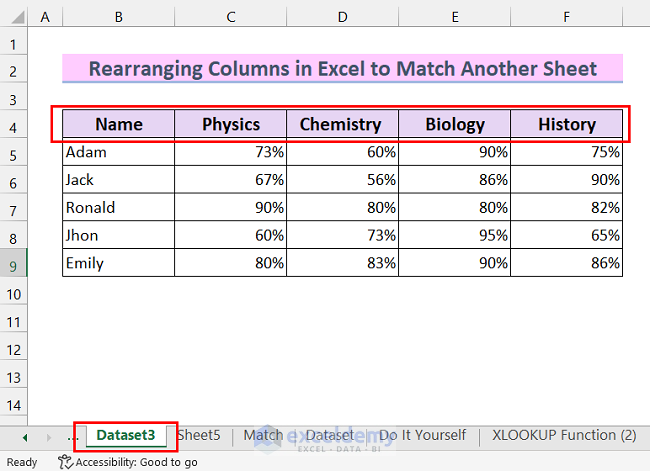
Here, I want to match the column order of the sheet “XLOOKUP Function” with the column order of the sheet “Dataset3”

Let me show you how to rearrange columns in Excel to match another sheet by using the XLOOKUP function step by step.

Steps:

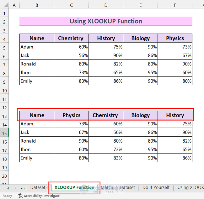
• To begin with, Insert the new column order in the sheet you want to rearrange the columns. Here, I have inserted the column order from “Dataset3” sheet into Row13 of the “XLOOKUP Function” sheet.
  

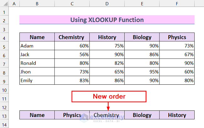
• Next, select the cell from where you want to rearrange your data according to the column order. Here, I have selected cell B14
• After that in the B14 type, the formula is shown below,

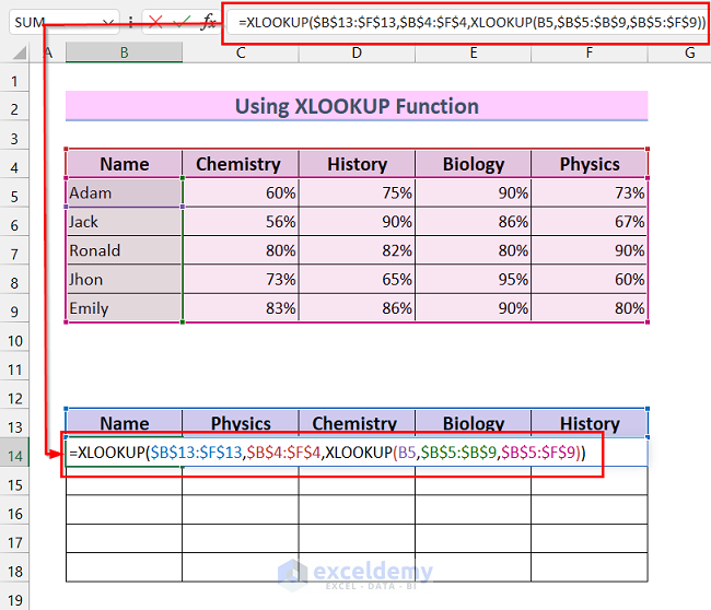
Here, in the XLOOKUP function, I selected cell range B13:F13 as lookup_value, and B4:F4 as lookup_array. Next, as a return_array I used another XLOOKUP function. Where, I selected the cell B5 as lookup_value, B5:B9 as lookup_array, and B5:F9 as return_array.
In every case, I used absolute cell reference so that the selected range remain the same while using the AutoFill.

Now, the XLOOKUP function will give you the results for the B5 cell from the return_array.

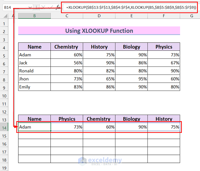
• Press ENTER key and you will see that the data are rearranged according to the new order.

• After that, you can use the Fill Handle tool to AutoFill the formula for the rest of the cells. That will give you the results accordingly.

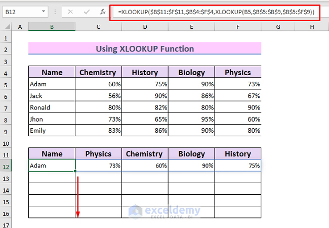
• Now you will see that all the data are sorted according to the new order.

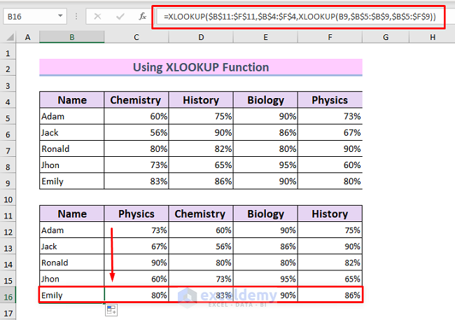
• Finally, we have got our desired table according to the order of the sheet named “Dataset3”.

In this method, you can rearrange your columns to match another sheet without losing the original arrangement.

4. Using MATCH Function to Rearrange Column Values

By using the MATCH function, you can rearrange the data of a column to match another sheet.

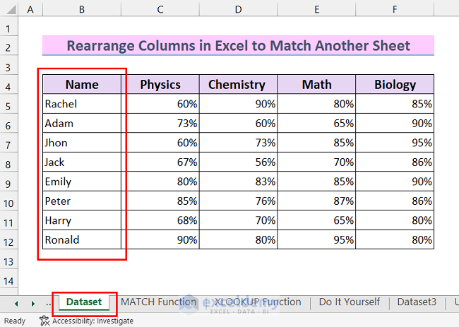
For this method, I want to rearrange the order of the Name column from the sheet “MATCH Function” to match the order of the name column of the sheet “Dataset”. 

Let’s learn how to rearrange columns in Excel to match another sheet using the MATCH function step by step.

Steps:

• Firstly, you have to Insert a new column in your sheet. Here, I have inserted a new column

I named it Helper Column.

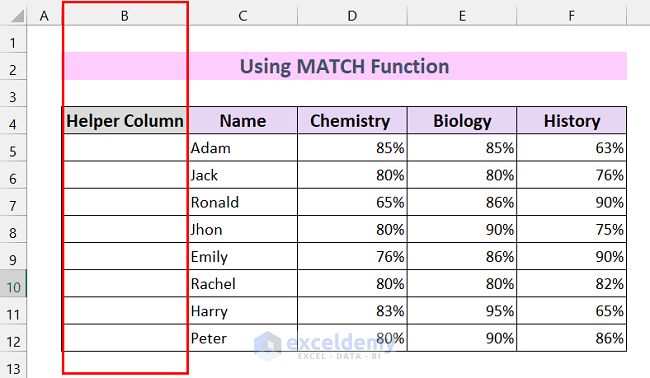
• Next, type the following formula in cell B5.

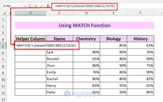
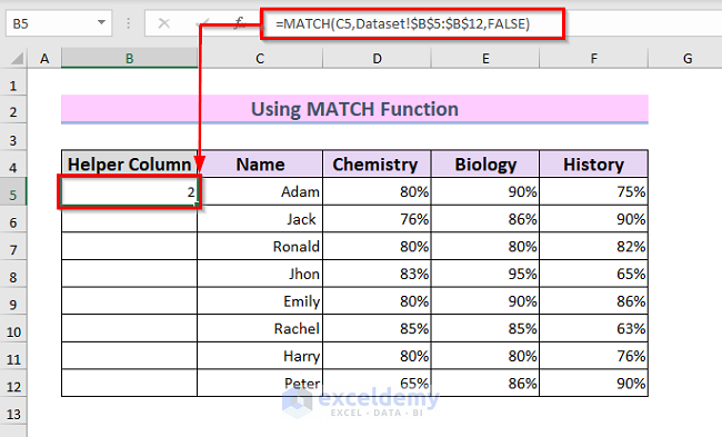
Here, in the MATCH function, I have selected C5 as lookup_value, and selected cell range Dataset!$B$5:$B$12 as lookup_array from Dataset sheet, and also selected FALSE as match_type. Now, this will return the order in which it matches with the lookup_array.

• After that, press ENTER and you will get the new sort order for the row.

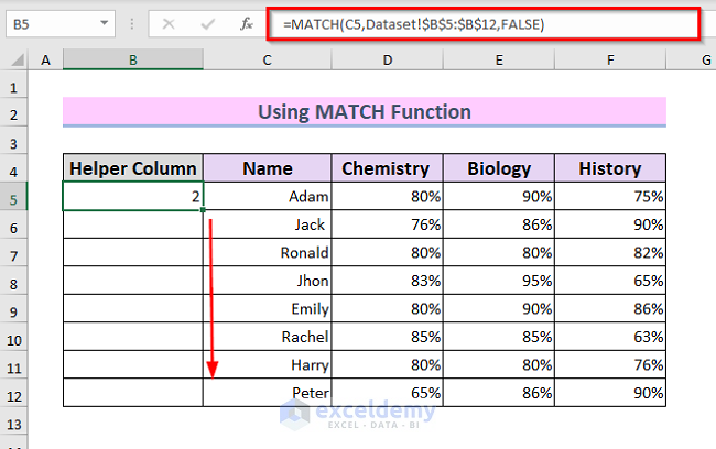
• Next, you can use the Fill Handle tool to AutoFill the formula for the rest of the cells.

• Now, you will get the Sorting order for the whole table.

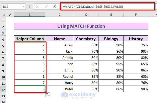
After getting the sort order, you will have to sort the rows using the Sort command.

• For that, you will have to select the range. Here, I selected the range B4:F12.
• And then, you will have to go to the Data tab >> select Sort from Sort & Filter.

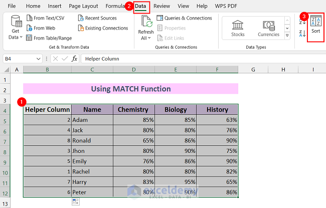
After that, the Sort dialog box will appear.

• Next, In that Sort dialog box click on Options and mark on Sort top to bottom and select Ok.

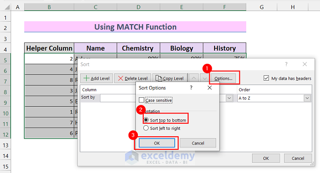
• And then, back in the Sort dialog box select the column in which you have inserted the sorting order in the Sort by menu. Here I have chosen the Helper Column.
• After that, select Smallest to Largest in the Order menu.
• Finally, select OK. That will sort your rows according to the order.

• Now, you can Delete the Helper Column and get your exact rearranged columns.

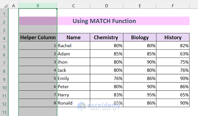
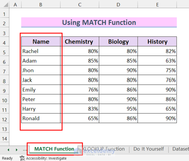
Here, you can see that all the columns in sheet “MATCH function” are rearranged according to the columns in sheet “Dataset”.

Read More: How to Rearrange Columns in Excel

Things to Remember

• While you are using the Sort command you will have to insert the column order carefully otherwise you will get the wrong column arrangement.
• For the drag and drop method, there can not be any merged cells. If you have any it will give you an error.

Practice Section

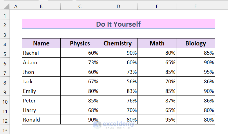
Here, I have given a practice sheet for you to practice different methods on how to rearrange columns in Excel to match another sheet.

Download Practice Workbook

Conclusion

In this article, I tried to cover 4 simple ways on how to rearrange columns in Excel to match another sheet. I hope this was helpful for you.  Most importantly we recommend you to practice more and more to get perfection. Last but not the least, if you have any suggestions or any other feedback feel free to let me know in the comment below.

Related Articles

• How to Rearrange Data in Excel
• How to Rearrange Columns Alphabetically in Excel

<< Go Back to Rearranging in Excel | Data Analysis with Excel | Learn Excel