How to Rearrange Data in Excel (5 Examples)

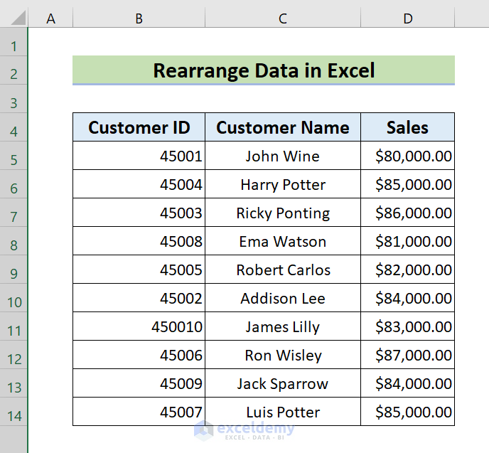
Below is a dataset containing information on a department store in three columns: Customer ID, Customer Name, and Sales.

Method 1 – Using the Transpose Command

Steps:

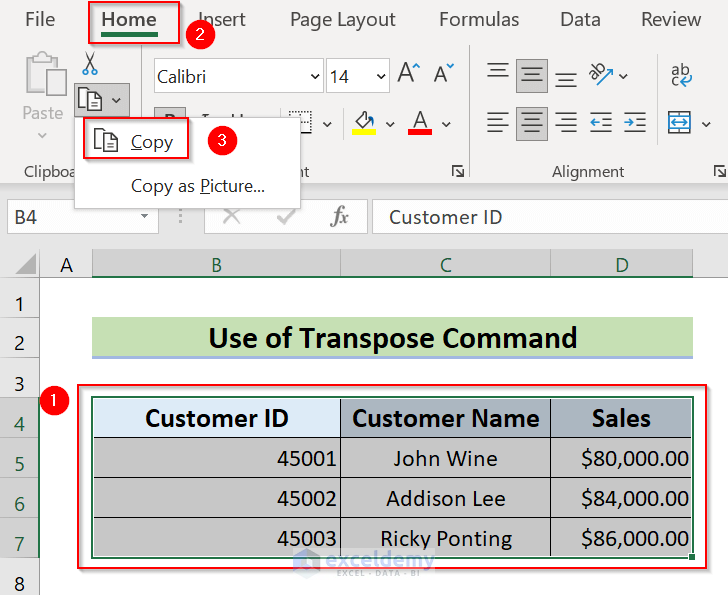
• Select the data that we want to rearrange. Here, I selected the range B4:D7.
• Go to the Home tab >> Select Copy

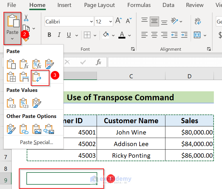
• Select a cell where you want to keep the rearranged data. Here, I select the B9 cell.
• From Paste group >> choose Transpose.

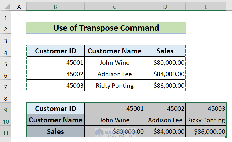
We can see the Rearranged Data.

Method 2 – Applying the Power Query 

Let’s use the following dataset: Customer ID in column B and Customer Name, Sales, Profit in column C.

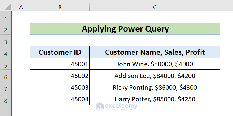
Steps:

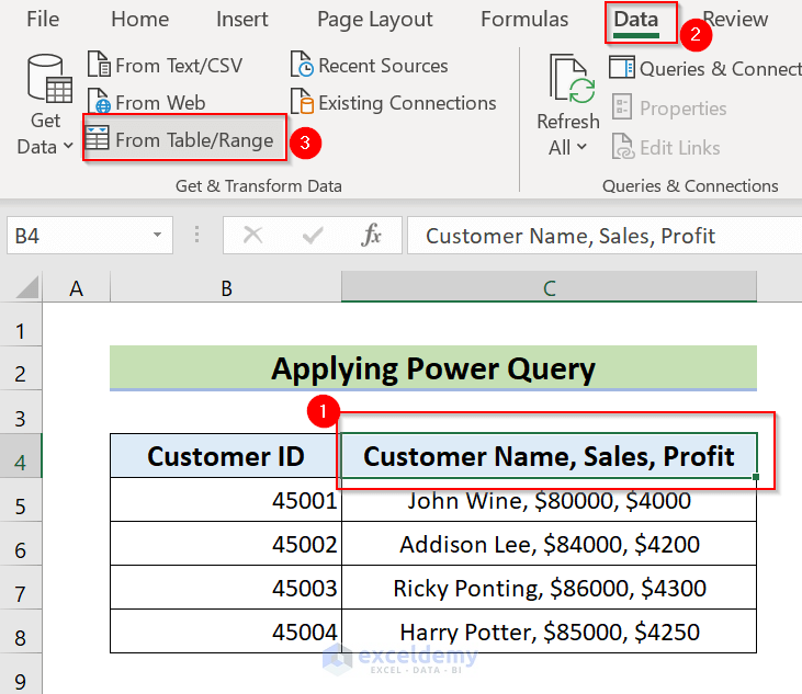
• Select cell C4.
• Go to the Data tab >> choose From Table/Range.

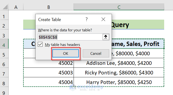
A dialog box of Create Table will appear.

• Select the data for your table. Here, I selected the range B4:C8.
• Make sure that “My table has headers” is marked.
• Press OK.

We will see the Power Query column.

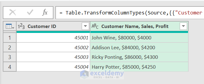
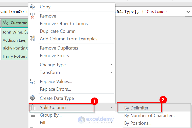
• Right-click on the Customer Name, Sales, Profit column.
• Go to Split Column >> choose By Delimiter.

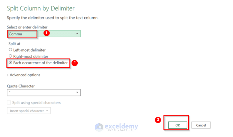
• Select Comma as Delimiter.
• From “Split at,” select Each occurrence of the delimiter.
• Press OK.

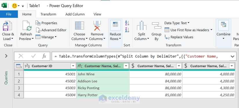
We will see the following table.

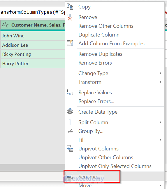
• Right-click on the 2ndColumn  >> select Rename.

• We will get the following table by following the same procedure for other columns.

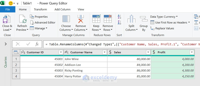
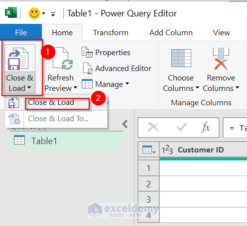
• From Close & Load >> select Close & Load.

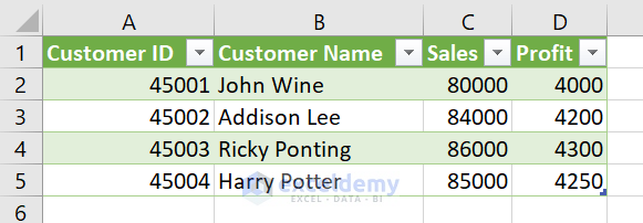
We will see the rearranged Data Table.

Method 3 – Using a Keyboard Shortcut to Rearrange a Single Column

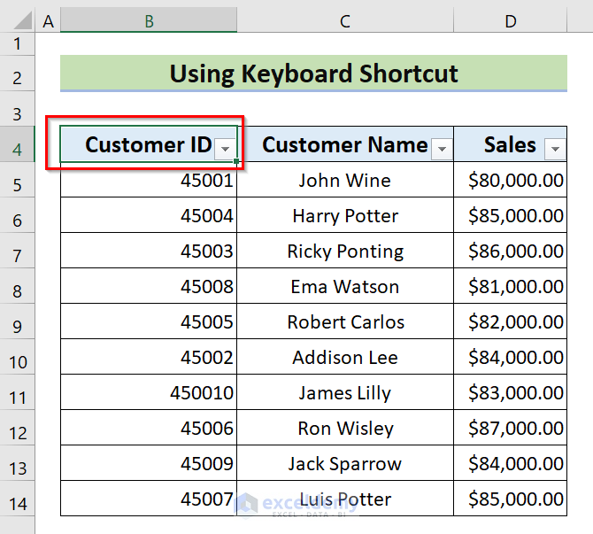
We are going to use the following dataset.

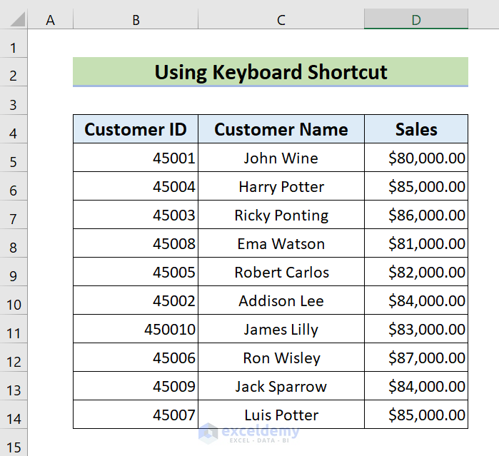
Steps:

• Select cell B4 (Customer ID).
• Press CTRL + SHIFT + L to Filter the dataset.

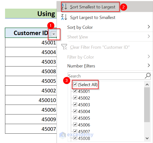
• Click on the filter icon >> select Sort Smallest to Largest >> choose (Select All).

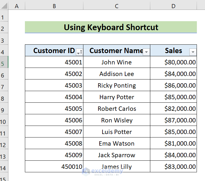
We will see the rearranged Data.

Read More: How to Rearrange Columns in Excel

Method 4 – Rearranging Data in Excel Table

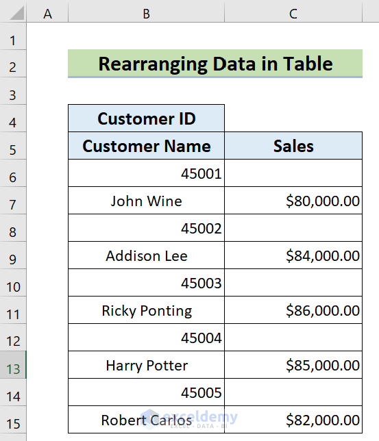
We will use the following dataset.

Steps:

• Select a different cell (F5) where you want to Rearrange the Data.
• Enter the corresponding formula in cell F5:

• Press ENTER to bring the value of cell B6 to cell F5.

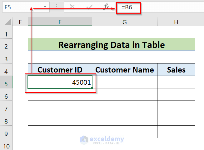
• We must do this up to two rows of our table to link with the given dataset.

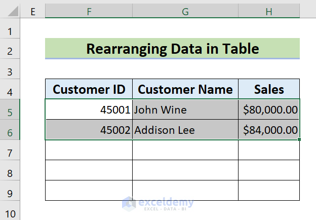
• Select those two rows.
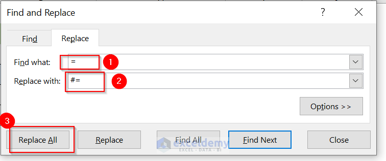
• Press CTRL+H to bring the Find and Replace dialog box.
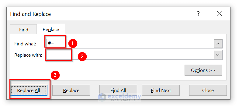
• Insert “=” in the “Find what” box and then insert “#=” in the “Replace with” box.
• Click on Replace All.

• We will see the following changes.
• Drag the Fill Handle icon to AutoFill the corresponding data in the rest of the cells.

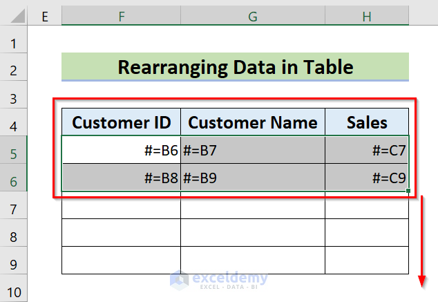
We will see the following table.

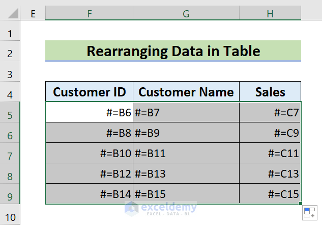
• Press CTRL+H to bring the Find and Replace dialog box again.
• Type “#=” in the “Find what” box and type “=” in the “Replace with” box.
• Click on Replace All.

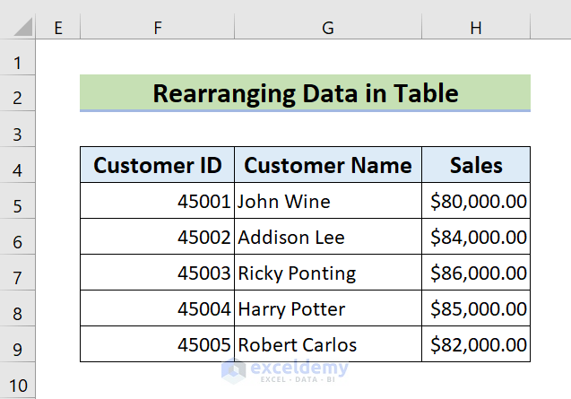
We will see the Rearranged Data in the table form.

Read More: How to Automatically Rearrange Columns in Excel

Method 5 – Applying the Sort Command to Rearrange Data

We will use the following dataset.

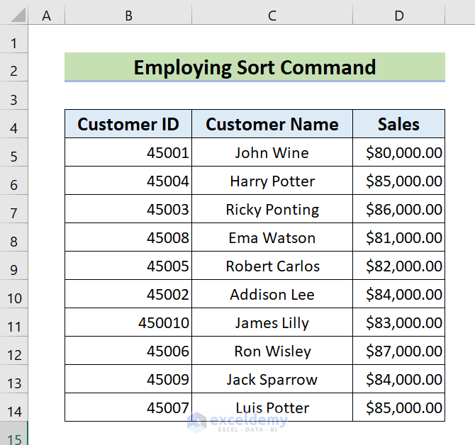
Steps:

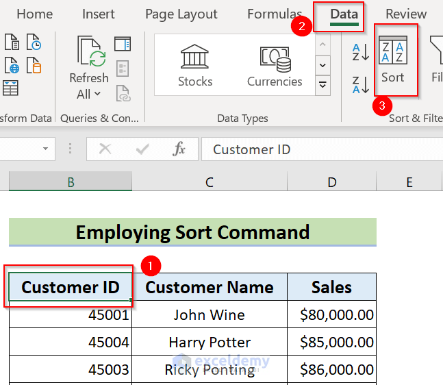
• Select the Customer ID column.
• Go to the Data tab >> choose Sort.

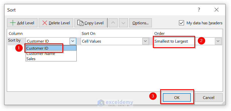
• Select “Customer ID” in the “Sort by” box >> “Smallest to Largest” in the “Order” box.
• Click on “OK”.

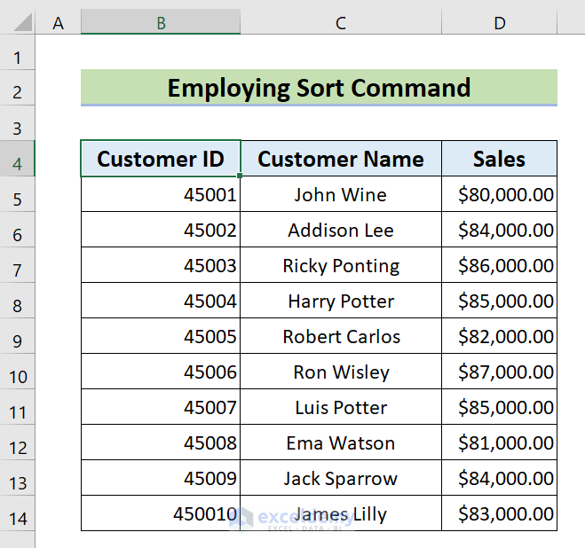
We will see the following rearranged Data.

Read More: How to Rearrange Columns in Excel

Things to Remember

• In the Rearranging data table method, we have to select the cells first then we will get the Find and Replace box.
• When you want to rearrange any data by column, then the Sort command or Keyboard shortcut methods will be more convenient for you.
• If you want to change the alignment of data, then the Transpose command will be preferable.
• When you have mixed data in a single column and you want to separate those into different columns, applying Power Query will be preferable.

Download the Practice Workbook

You can download the practice workbook from here:

Related Articles

• How to Rearrange Columns in Excel to Match Another Sheet
• How to Rearrange Columns Alphabetically in Excel

<< Go Back to Rearranging in Excel | Data Analysis with Excel | Learn Excel