Method 1. Finding Duplicate Values to Reconcile Data
To find the duplicate values and reconcile data:
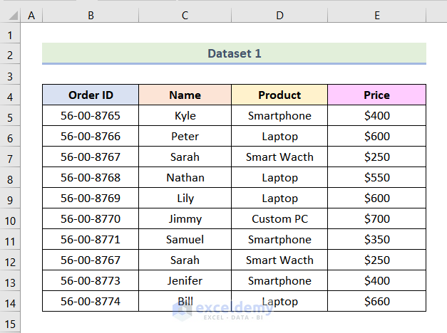
Step 1 – Finding the Duplicates
- Create an additional column: Duplicate Check.
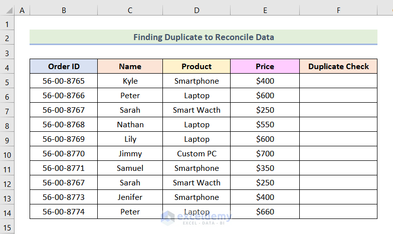
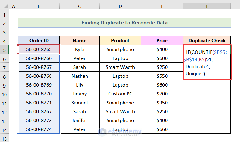
- Enter the following formula in F5.
=IF(COUNTIF($B$5:$B$14,B5)>1,"Duplicate","Unique")B5 represents the Order ID and $B$5:$B$14 indicates the array of the Order ID.
Formula Breakdown
- COUNTIF($B$5:$B$14,B5) → returns the number of occurrences of an item in a range. Here, $B$5:$B$14 is the range argument, and B5 is the criteria argument.
- Output → 1
- IF(COUNTIF($B$5:$B$14,B5)>1,”Duplicate”,”Unique”) → if the output of the COUNTIF function is larger than 1, it is a Duplicate value. Otherwise, it is a Unique value.
- Press ENTER.
Note: An absolute cell reference is used.
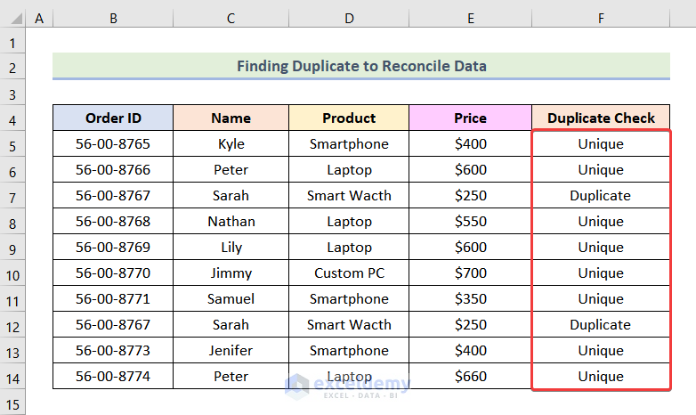
This is the output.
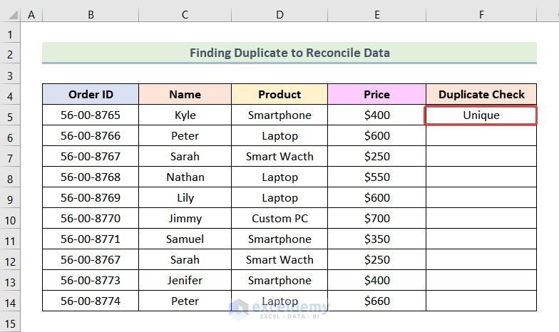
- Drag down the Fill Handle to see the result in the rest of the cells.
Step 2 – Using Conditional Formatting to Highlight the Duplicates
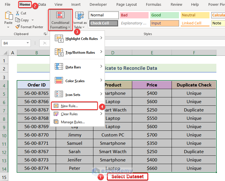
- Select the dataset and go to the Home tab.
- Click Conditional Formatting.
- Choose New Rule.
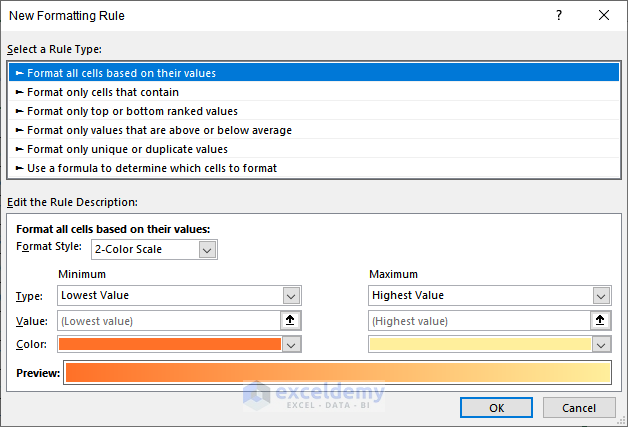
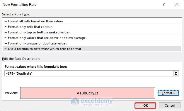
The New Formatting Rule dialog box will be displayed:
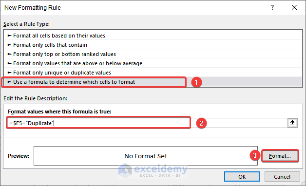
- Click Use a formula to determine which cells to format.
- Enter the following formula in Format values where this formula is true:.
=$F5="Duplicate"F5 refers to the Duplicate Check column.
- Click Format and choose a formatting.
- Click OK.
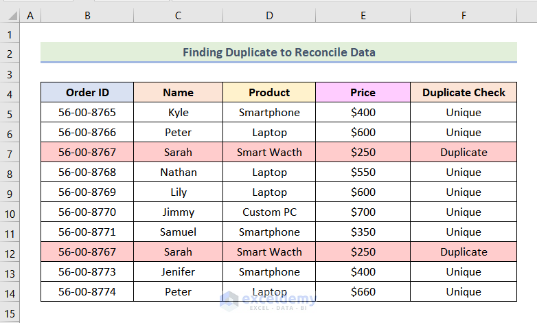
The Duplicate values are highlighted:
Read More: How to Do Reconciliation in Excel
Method 2 – Using the Table Format to Reconcile Data in Excel
Steps:
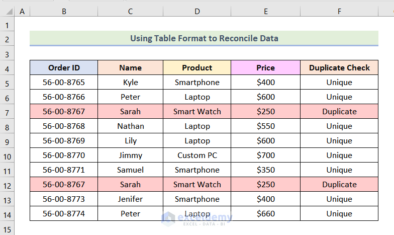
- Follow the steps described in the previous method to see the following output.
- Select the dataset and press CTRL + T.
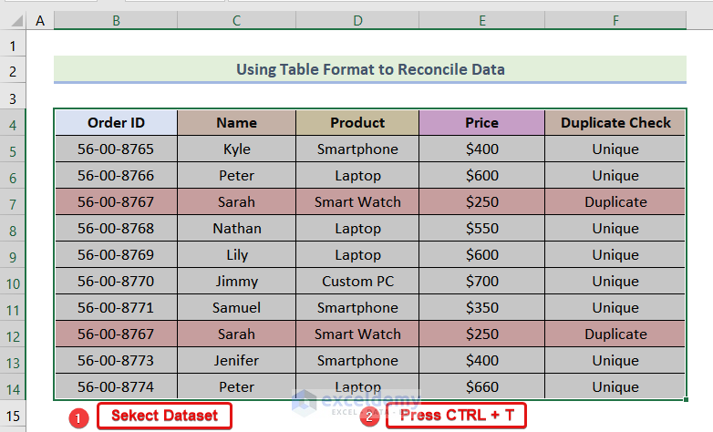
The Create Table dialog box will be displayed.
- Check My table has headers.
- Click OK.
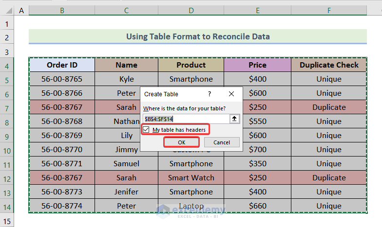
Your data will be converted into a table:
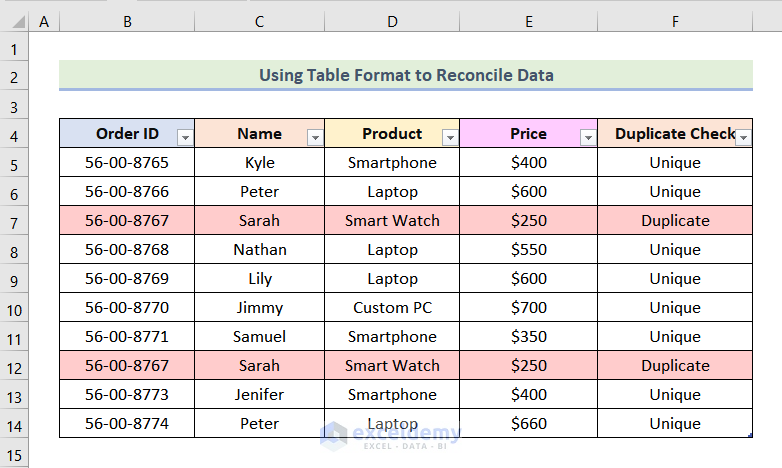
- Click the drop-down icon beside the Duplicate Check column.
- Uncheck Unique.
- Click OK.
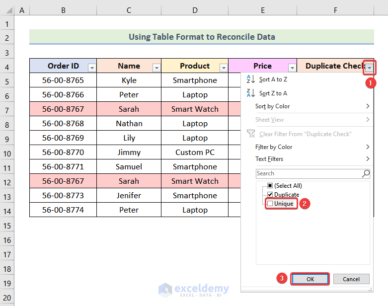
Only the duplicate values will be displayed.

Read More: How to Reconcile Two Sets of Data in Excel
Method 3 – Using Excel Functions to Reconcile Data
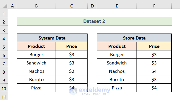
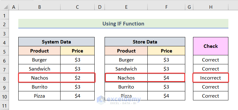
The following dataset showcases System Data and Store Data of prices in a restaurant. To check if there is any mismatch in the prices between System Data and Store Data:
3.1 Utilizing the MATCH Function
Steps:
- Create an extra column (Check).
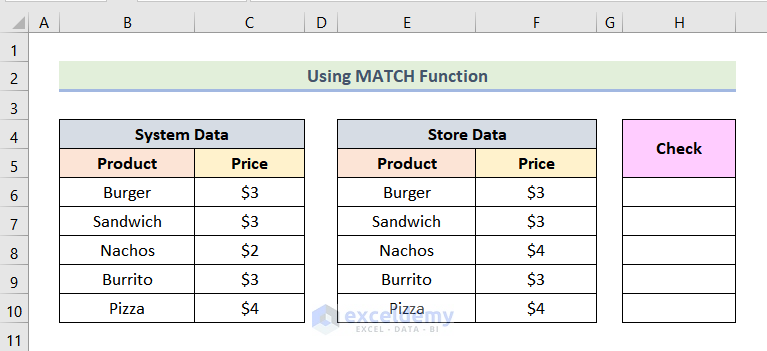
- Enter the formula below in H6.
=ISNUMBER(MATCH(F6,C6,0))F6 is the Price in Store Data and C6 is the Price in System Data.
Formula Breakdown
- MATCH(F6,C6,0) → returns the relative position of an item in an array that matches a supplied value in a defined order. Here, F6 is the lookup_value argument, C6 is the lookup_array argument, and 0 indicates the match_type argument.
- Output → 1
- =ISNUMBER(MATCH(F6,C6,0)) → it becomes
- =ISNUMBER(1) → The ISNUMBER function checks whether a cell value is a number or not and returns TRUE or FALSE as output.
- Output → TRUE.
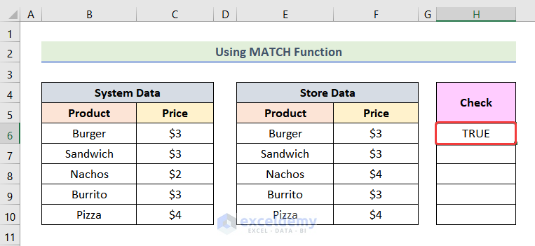
- Press ENTER.
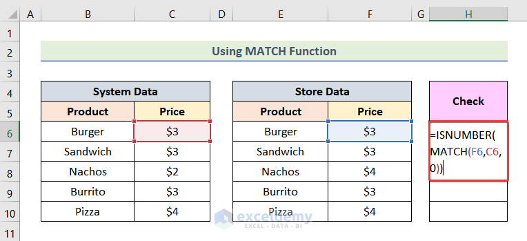
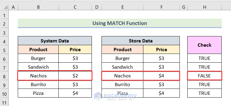
This is the output.
- Drag down the Fill Handle to see the result in the rest of the cells.
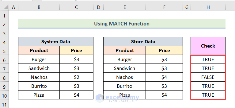
The Price of Nachos doesn’t match in System Data and in Store Data. The Check column returns FALSE.
3.2 Using the IF Function
Steps:
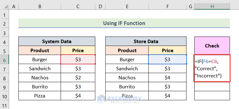
- Enter the formula below in H5.
=IF(F6=C6,"Correct","Incorrect")- Press ENTER.
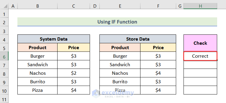
This is the output.
- Drag down the Fill Handle to see the result in the rest of the cells.
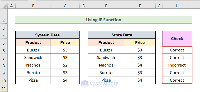
The Price of Nachos doesn’t match in System Data and in Store Data. The Check column returns Incorrect.
Method 4 – Reconciling Data for Bank Statements
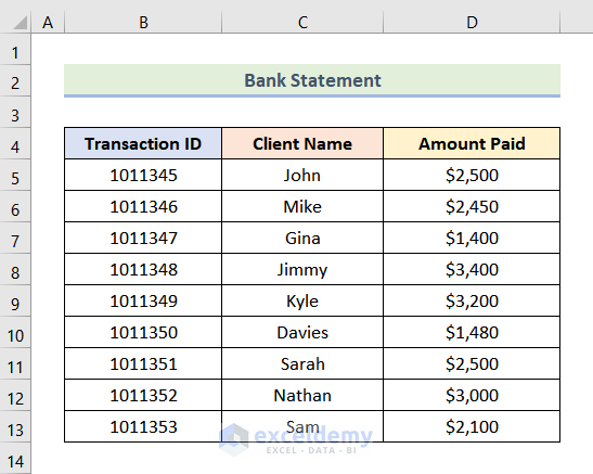
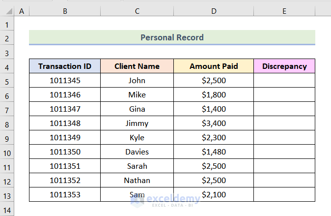
The following dataset showcases a Bank Statement of a company with amounts paid to different Clients. The company also keeps a Personal Record. To find if there is any Discrepancy between these two sets of data.
Step 1 – Finding the Discrepancy
- In the Personal Record worksheet, create an additional column named Discrepancy.
- Enter the formula below in E5.
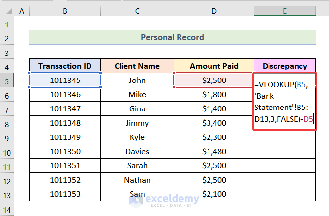
=VLOOKUP(B5,'Bank Statement'!B5:D13,3,FALSE)-D5B5 refers to the Transaction ID, D5 represents the Amount Paid, and B5:D13 denotes the array in Bank Statement.
Formula Breakdown
- VLOOKUP(B5,’Bank Statement’!B5:D13,3,FALSE) → checks for a value in the left-most column and returns a value from a specified column in the same row. B5 is the lookup_value argument, ‘Bank Statement’!B5:D13 is the table_array argument, 3 is the column_index_number argument, and FALSE indicates an exact match.
- Output → $2,500
- VLOOKUP(B5,’Bank Statement’!B5:D13,3,FALSE)-D5 → it becomes
- $2,500 – D5
- Output → $0
- Press ENTER.
This is the output.
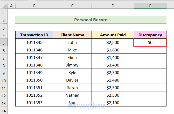
- Drag down the Fill Handle to see the result in the rest of the cells.
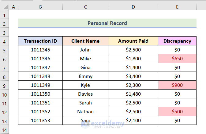
There are values greater than 0 in the Discrepancy column. Data in the Bank Statement and the Personal Record doesn’t match.
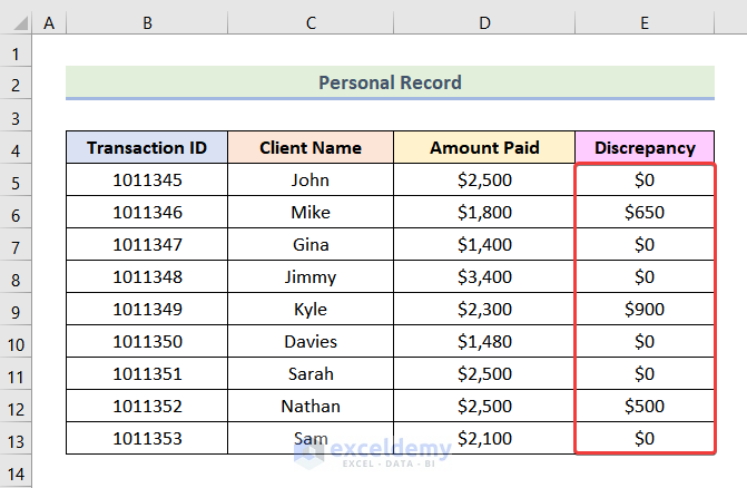
Step 2 – Highlighting the Discrepancy
- Select the dataset and go to the Home tab.
- Select Conditional Formatting.
- Choose Highlight Cells Rules.
- Click Greater Than.
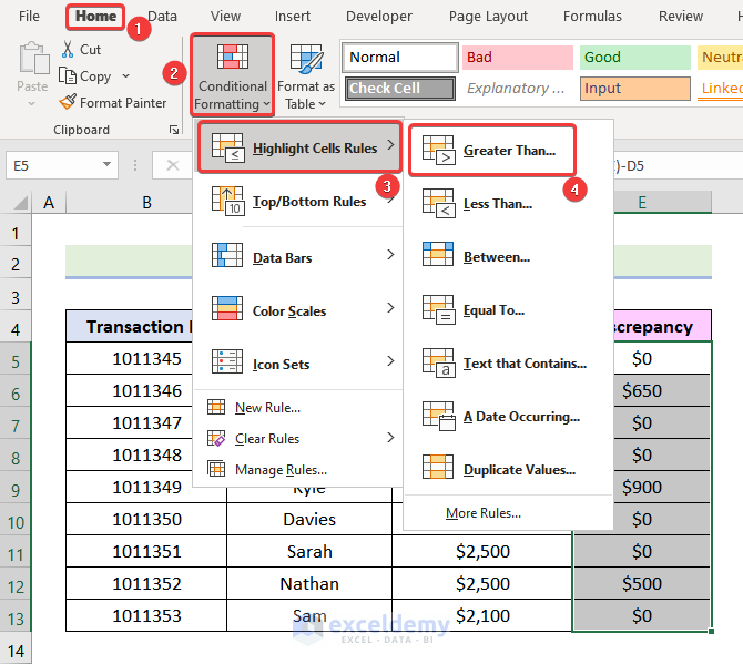
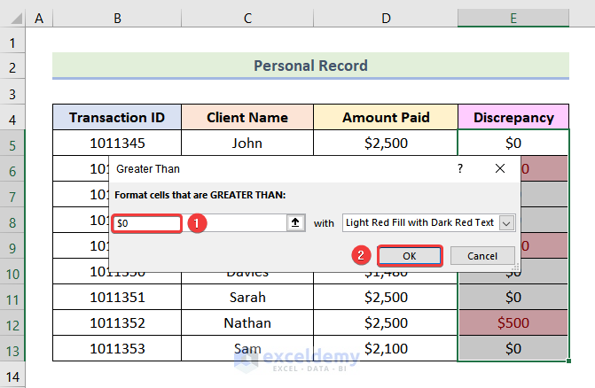
The Greater Than dialog box is displayed.
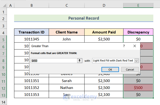
- Enter $0 in Format cells that are GREATER THAN:.
- Click OK.
Values that are greater than 0 in the Discrepancy column are highlighted.
Read More: Automation of Bank Reconciliation with Excel Macros
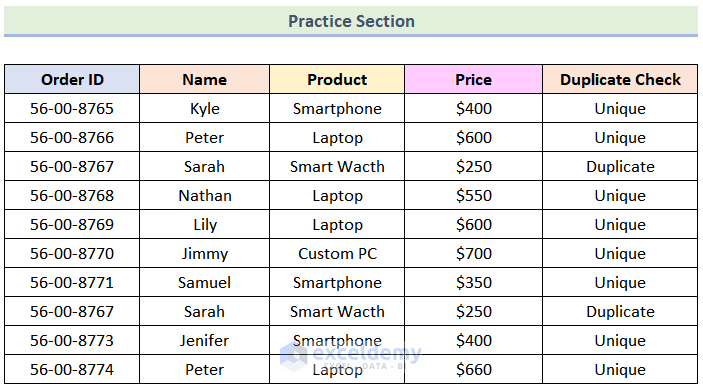
Practice Section
Practice here.
Download Practice Workbook
Related Articles
- How to Do Intercompany Reconciliation in Excel
- How to Reconcile Vendor Statements in Excel
- How to Reconcile Data in 2 Excel Sheets
- How to Perform Bank Reconciliation Using VLOOKUP in Excel
- How to Reconcile Credit Card Statements in Excel
<< Go Back to Excel Reconciliation Formula | Excel for Accounting | Learn Excel
Get FREE Advanced Excel Exercises with Solutions!

