How to Remove Asterisk in Excel (5 Simple Methods)

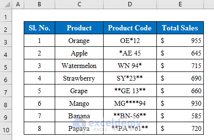
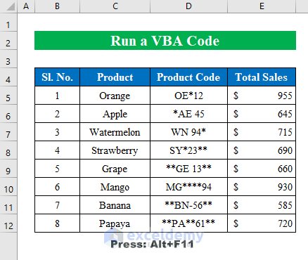
Suppose we have a dataset of a fruit shop containing columns for Product, Product Code, & Total Sales. We will remove the asterisk sign from the Product Code column and place it in a different position.

Method 1 – Using the Find & Replace Command

Steps:

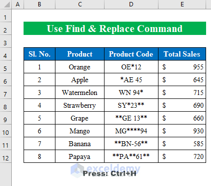
• Select any cell in the dataset and press Ctrl+H to open the “Find & Replace” window.

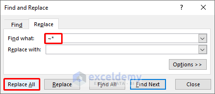
• In the “Find what” section, type the tilde & asterisk sign (~*).
• Click “Replace All” to continue.

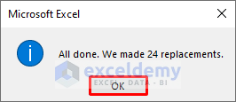
A confirmation window will appear confirming the replacement.

• Click OK.

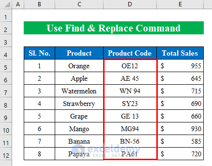
All the asterisks from the worksheet are removed.

Read More: How to Remove Apostrophe in Excel

Method 2 – Using the SUBSTITUTE Function

The SUBSTITUTE function replaces a specific text from a given string.

Steps:

• Choose a cell to apply the formula, here cell G5.
• Enter the following formula:

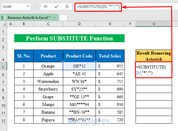
• Press Enter to get the output in the cell.
• Pull the “Fill Handle” down to fill up the cells below.

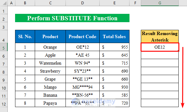
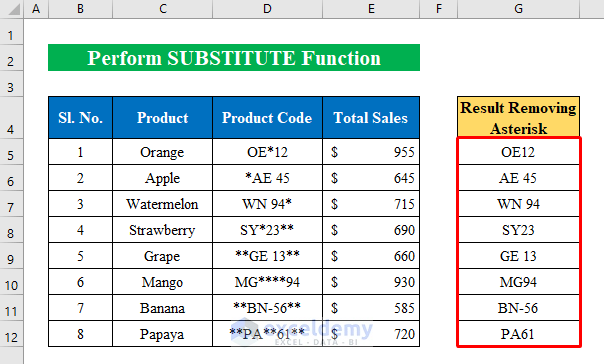
• All the asterisks (*) are removed from the column, even when they are in different positions.

Read More: How to Remove Non-Alphanumeric Characters in Excel

Method 3 – Combining the TRUNC and SUBSTITUTE Functions to Remove Asterisk from Numbers Only

In those previous methods, we have removed asterisks from texts. Now we’ll remove the asterisk (*) from numbers.

Suppose we have a dataset of some Employee Names & IDs. In the Employee ID column are various asterisks. Let’s remove those with the help of functions.

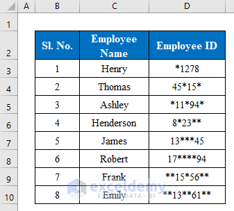
Steps:

• In cell F5, enter the following formula:

The TRUNC function returns a truncated number based on the given number of digits.

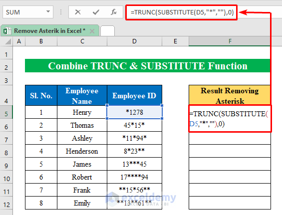
• Press Enter.
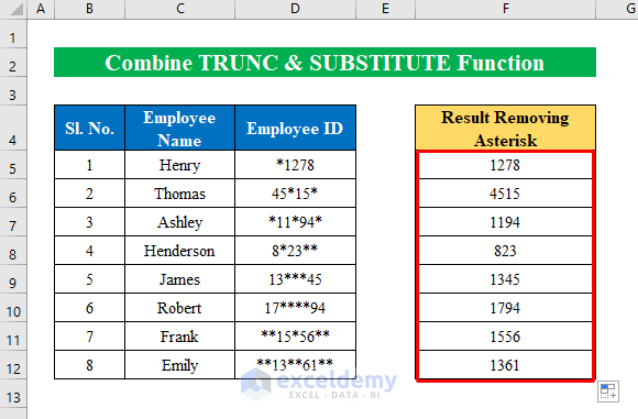
• Drag the “Fill Handle” down.

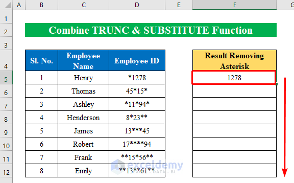
All the asterisks are removed from the numbers.

Method 4 – Using SUMPRODUCT and SUBSTITUTE Functions to Remove Asterisk from Numbers

An alternative method to remove asterisks from numbers is with the SUBSTITUTE function, which will substitute the asterisk sign from the cells, and then the SUMPRODUCT function which will return the total values of a cell.

Steps:

• In cell F5, enter the following formula:

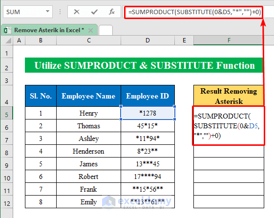
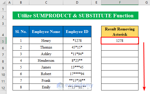
• Press Enter.
• Pull the “Fill Handle” down to get the result in all cells.

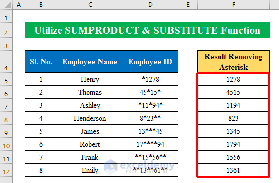
Regardless of where they were positioned in the numbers, the asterisks are removed.

Method 5 – Using Excel VBA Code

Steps:

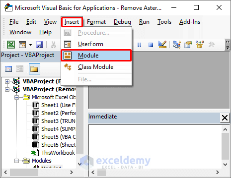
• Press Alt+F11 to open the “Microsoft Visual Basic for Applications” window.

• Go to “Module” from the “Insert” option.

• Place the following code in the module that opens, then click “Run”:

Sub Find_andReplace()
Dim stringPC As String
stringPC = "OE*12, *AE 45, WN 94*, SY*23**, **GE 13**, MG****94, **BN-56**, **PA**61**"
stringPC = Replace(stringPC, "", " ")
MsgBox stringPC
End Sub

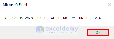
• In the output MsgBox are the requested results, with all the asterisks from the dataset removed.

Things to Remember

• When using the “Find & Replace” feature, don’t forget to put the tilde(~) sign before the asterisk sign in the “Find what” section. Otherwise, you will lose all the dataset texts and numbers from the worksheet.

Download Practice Workbook

Related Articles

• How to Remove Parentheses in Excel
• How to Remove Semicolon in Excel
• How to Remove Dashes in Excel
• How to Remove Dashes from Phone Number in Excel
• How to Remove Dashes from SSN in Excel
• How to Remove Non-Printable Characters in Excel 

<< Go Back To Remove Specific Characters in Excel | Excel Remove Characters | Data Cleaning in Excel | Learn Excel