How to Remove Partial Data from Multiple Cells in Excel (6 Methods) -

Dataset Overview

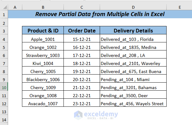
To make the explanation clear, we’ll use a dataset representing product information from a fruit shop, but some information is condensed. The dataset consists of three columns: Product & ID, Order Date, and Delivery Details.

Method 1 – Using Flash Fill to Remove Partial Data from Multiple Cells

If your dataset contains condensed values, you can utilize the Flash Fill command to remove partial data from multiple cells in Excel.

To use the Flash Fill command, you first need to establish a pattern to follow.

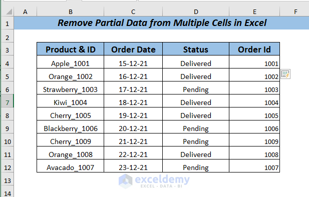
For example, you can create a pattern for the delivery Order ID by removing the Product part from the Product & ID column.

Navigate to the Data tab and select Flash Fill.

The partial data from the Product & ID column will be removed based on the established pattern.

Method 2 – Using the Find & Replace Feature

If you need to remove specific data partially from multiple cells, the Find & Replace feature proves incredibly helpful.

Navigate to the Home tab, locate the Editing group and under Find & Select, choose Replace.

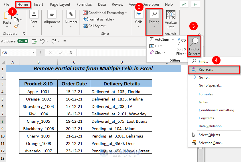
This action will prompt a dialog box for Find and Replace.
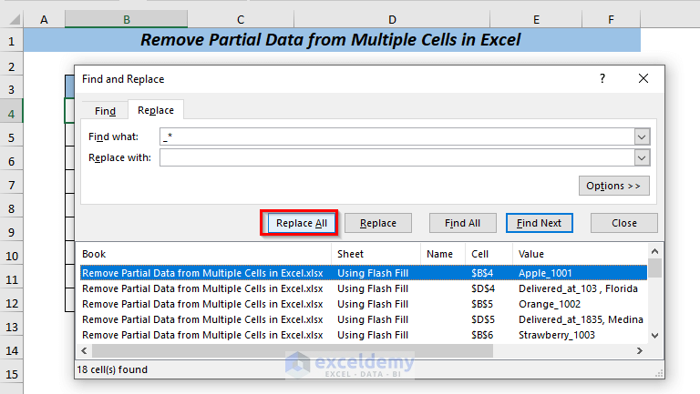
In the Find what field, enter the character you wish to locate and remove.
We’ve entered the character (_*) in the Find what field. We’ve appended an asterisk (*) after the underscore (_) to target only the Product name and delivery Status from their respective columns, Product & ID and Delivery Details.
Since we solely require the Product name and delivery Status, we’ve left the Replace with field blank.
Click on Find All.

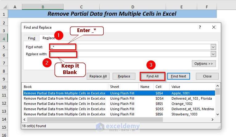
This will display which cell values contain the specified character.

Proceed with clicking Replace All.

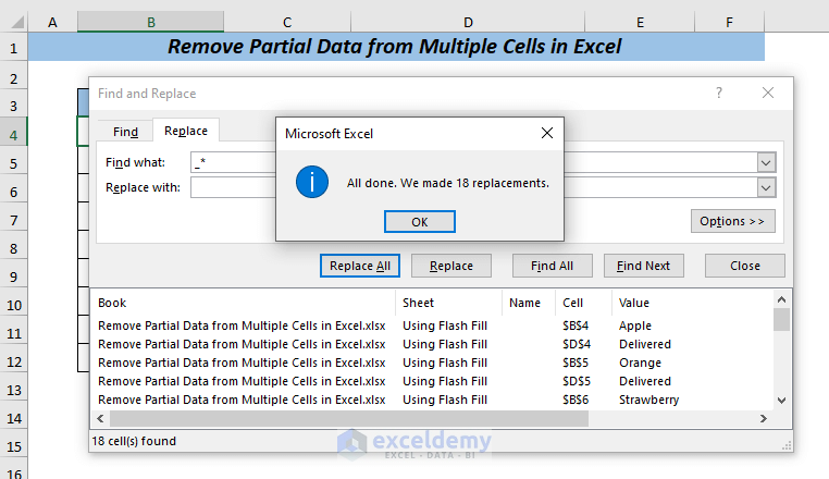
A notification indicating the number of replacements made will appear.

In this case, it will indicate 18 replacements.

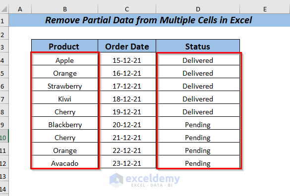
You’ll obtain the Product name and delivery Status from their respective columns, Product & ID and Delivery Details.

Read More: How to Clean Up Raw Data in Excel

Method 3 – Utilizing the Text to Columns Option

One of the most effective methods for removing partial data from multiple cells is through the Text to Columns command. This command can be accessed from the ribbon.

To get started, follow these steps:

Select the cell range from which you wish to remove partial data.
For example, we’ve selected cell range B4:B12.
Navigate to the Data tab, then select Text to Columns.

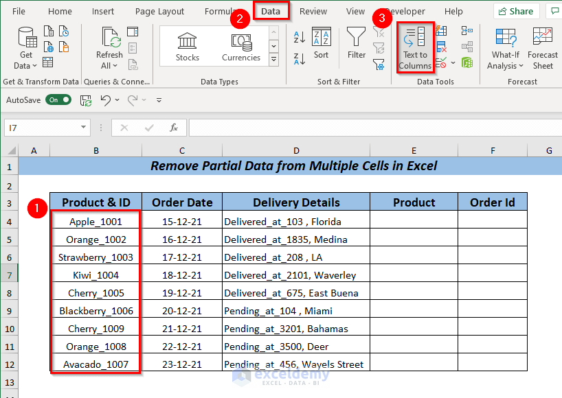
This action will prompt a dialog box to appear.

Choose the appropriate data type.

Select Delimited and then clicked Next.

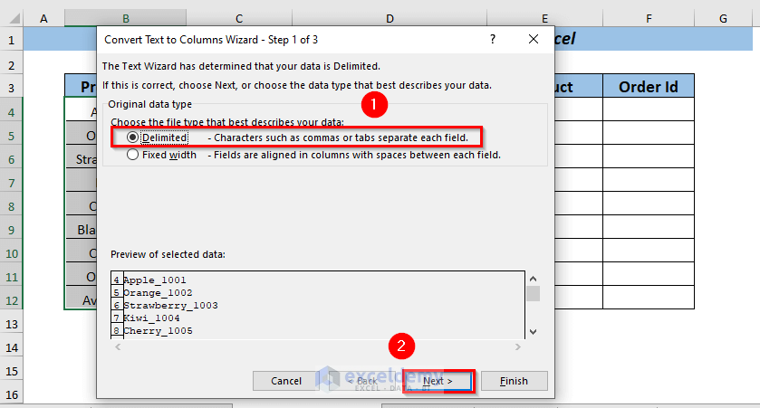
Another dialog box will appear.

Here, specify the Delimiters present in your data.

Selected the underscore (_) under the Other option, as this character is present in your data.

If desired, preview how your data will be split in the Data preview section.

Click Next again.

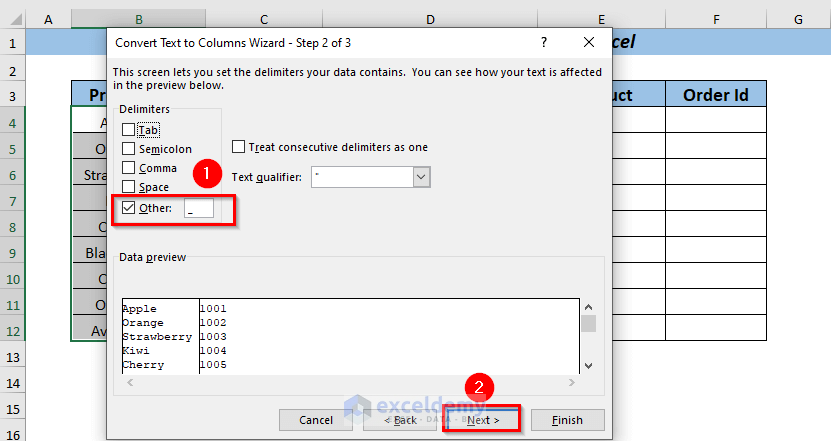
Once more, a dialog box will appear.

From here, select the destination where you want to place the separated data.

We chose cell E4.
Click Finish.
Another dialog box will pop up.

From there, select the destination of your choice to place the separated data.

We selected the E4 cell.
Click Finish.

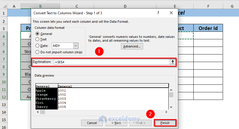
You’ll notice the data from the Product & ID column has been separated into two new columns.

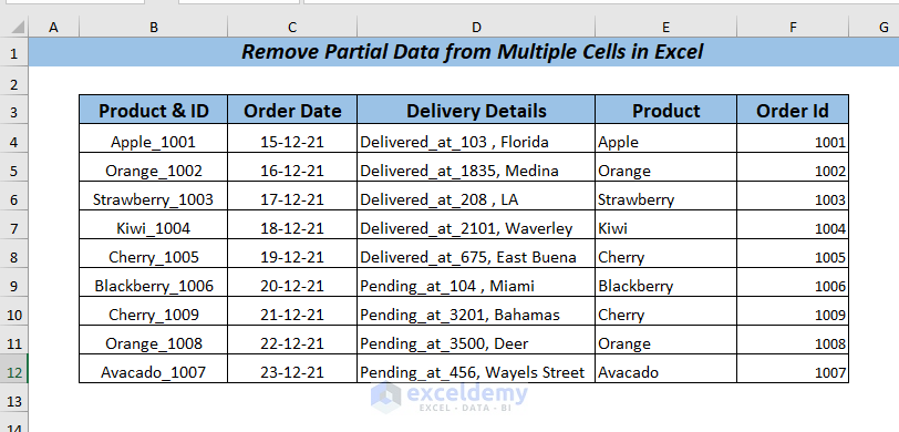
Now, you can delete any unnecessary parts of the data as needed.

Read More: How to Clean Survey Data in Excel

Method 4 – Utilizing the RIGHT Function to Remove Partial Data from Multiple Cells

The RIGHT function proves handy for removing partial data from multiple cells.

For instance, let’s say we want to extract only the Order ID from the Product & ID column using the RIGHT function.

Here’s how you can employ the RIGHT function:

First, designate a cell where you want the resultant value to appear.

We’ve chosen cell E4.

Next, enter the following formula either directly into the selected cell or into the Formula Bar:

=RIGHT(B4:B12, 4)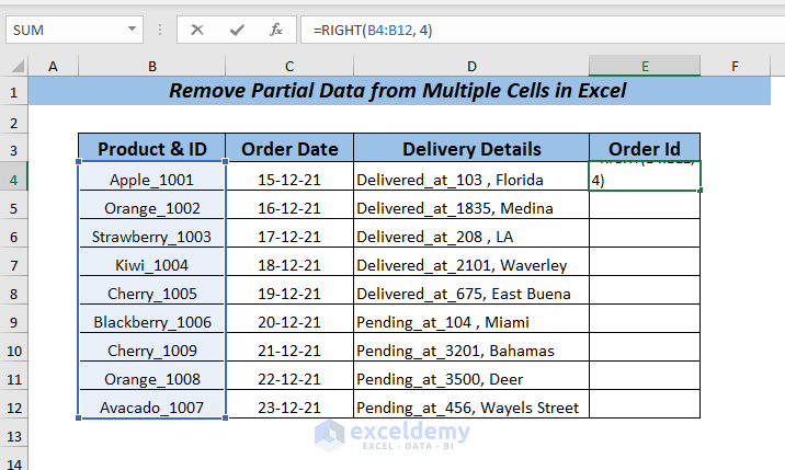

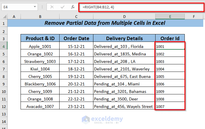
In this formula, the RIGHT function is applied to the cell range B4:B12 as text. The num_chars” parameter is set to 4, indicating that we want to extract four characters from the right.

Press ENTER. You’ll now obtain the right four characters for all selected cell ranges, which represent the Order ID.

Read More: Data Cleaning Techniques in Excel

Method 5 – Leveraging the LEFT & SEARCH Functions in Excel

The combination of the SEARCH function with the LEFT function offers another approach to remove partial data from multiple cells.

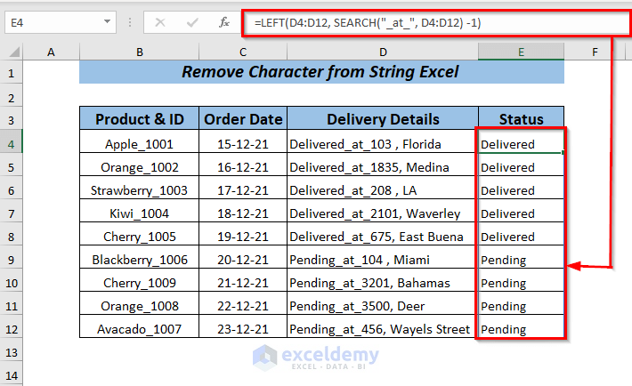
For instance, let’s say we want to extract only the left value, representing the delivery status, from the Delivery Details column using this method.

Here’s how you can proceed:

Begin by selecting a cell where you want the resultant value to appear.

We’ve opted for cell E4.

Enter the following formula either directly into the selected cell or into the Formula Bar:

You can also use the SEARCH function with the LEFT function to remove partial data from multiple cells.

=LEFT(D4:D12, SEARCH("_at_", D4:D12) -1)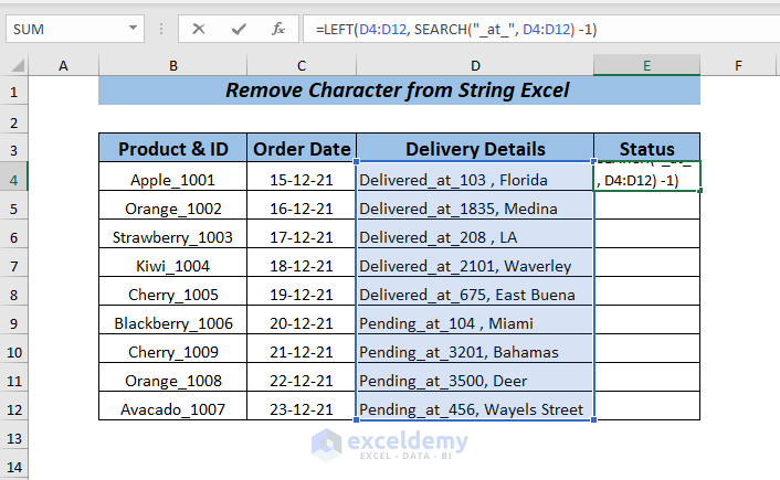

Formula Breakdown

- Here, the SEARCH function will search the given character _at_ as we used it as find_text. In the within_text selected the D4:D12 cell so that it searches the selected text within the given cell then subtracted 1 character.
- After getting the position number by using the SEARCH function, the LEFT function will use it as num_chars and also select the D4:D12 cell to extract the left value from the searched character.

Press the ENTER key.

Upon completion, you’ll obtain the partial data representing the delivery status from the Delivery Details column.

Method 6 – Utilizing the LEFT, FIND & SUBSTITUTE Functions in Excel

Using a combination of the FIND function and the SUBSTITUTE function within the LEFT function enables you to remove partial data from multiple cells.

For illustrative purposes, let’s extract partial data, specifically the Product & ID name, from the Order Info column using this method.

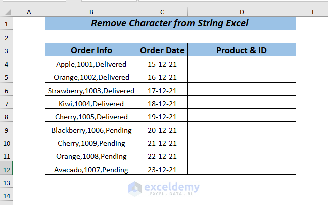
Here’s how to proceed:

Begin by selecting a cell where you want the resultant value to appear.

We’ve chosen cell E4.

Next, enter the following formula either directly into the selected cell or into the Formula Bar:

=LEFT(B4:B12,FIND("_",SUBSTITUTE(B4:B12,",","_",2))-1)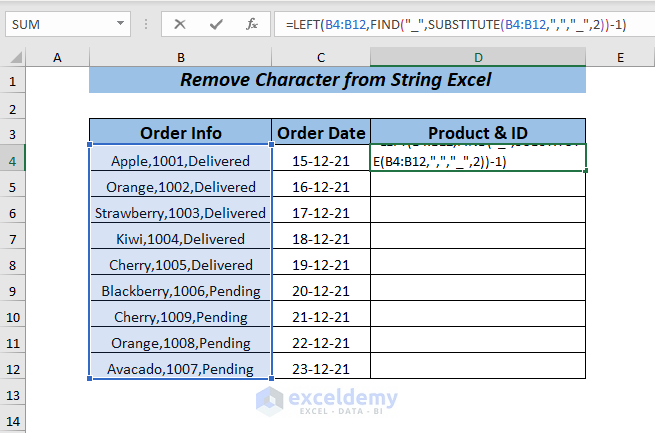

Formula Breakdown

- Here, the FIND function searches for the underscore (_) within the text provided (B4:B12). I’ve specified the underscore (_) as the find_text. Since the data contains multiple commas, the SUBSTITUTE function is utilized within the FIND function. It replaces the second comma (,) with an underscore (_) to avoid ambiguity.
- The FIND function then calculates the position of the substituted underscore (_) and subtracts 1 character from it.
- The LEFT function extracts the left value based on the position of the second comma (,) as the num_chars parameter. The cell range B4:B12 is selected to ensure extraction from the relevant cells.

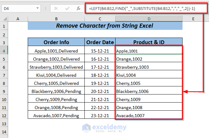
This approach is particularly useful when dealing with data containing multiple commas or any special characters.

➤ Press ENTER. You’ll now obtain the partial data representing the Product & ID from the Order Info column.

Practice Section

I’ve included a practice sheet in the workbook to help you apply the methods explained above. You can download it from the link provided below.

How to Remove Partial Data from Multiple Cells in Excel (6 Methods)