Method 1 – Remove Percentage Using General Format in Excel
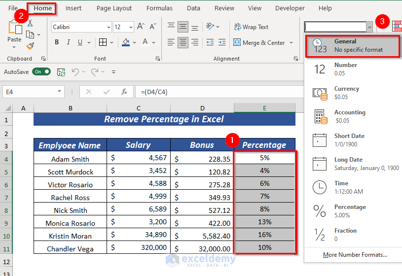
Select the cell or cell range from where you want to remove the percentage.
Open the Home tab >> from Number Format >> select General.
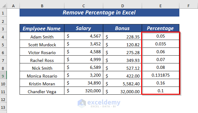
You will get the Percentage values in General format without a percentage sign.
Method 2 – Remove Percentage Using Number Format
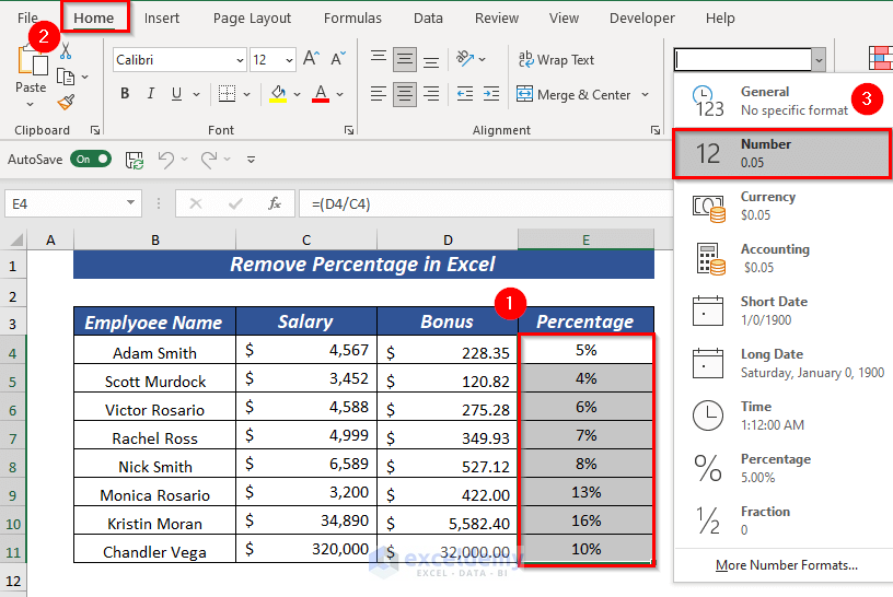
Select the cell or cell range from where you want to remove the percentage sign.
Open the Home tab >> from Number Format >> select Number.
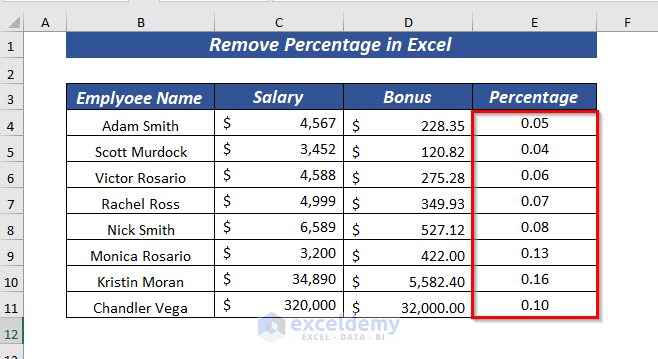
The Percentage values will be formatted as Numbers.
Method 3 – Remove Percentage Using Paste Special in Excel
Add an additional column and enter the value 100. To remove the percentage sign, multiply the value by 100.
The logic behind this is, (5.00/100)*100
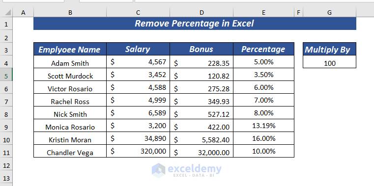
Select the cell where you kept the value 100.
Right-click and select Copy from the context menu.
You can also use CTRL + C to copy the value.
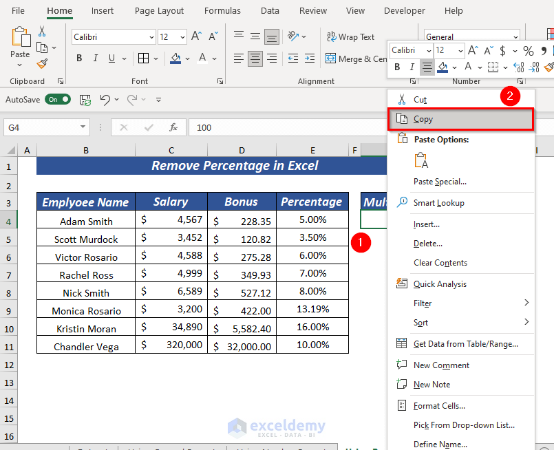
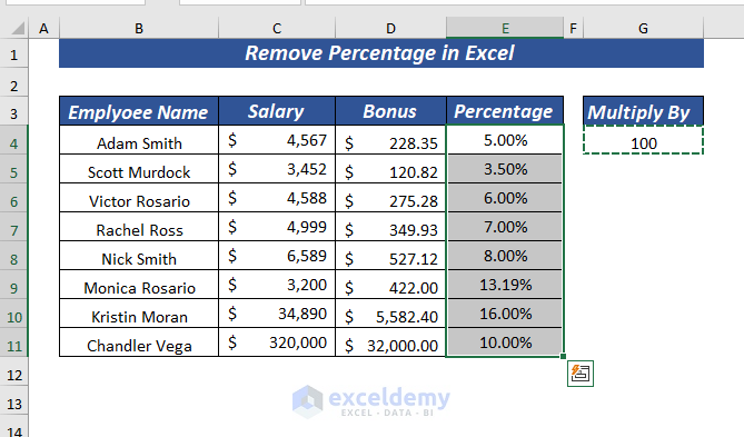
Select the cell or cell range from where you want to remove the percentage sign and keep the value as it is.
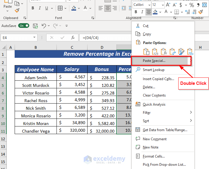
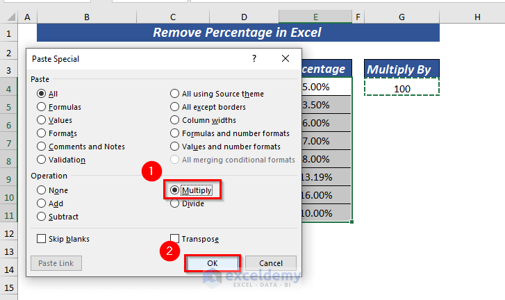
Right-click and double-click on Paste Special from the context menu.
⏩ Select Multiply from the Operation section.
Click OK.
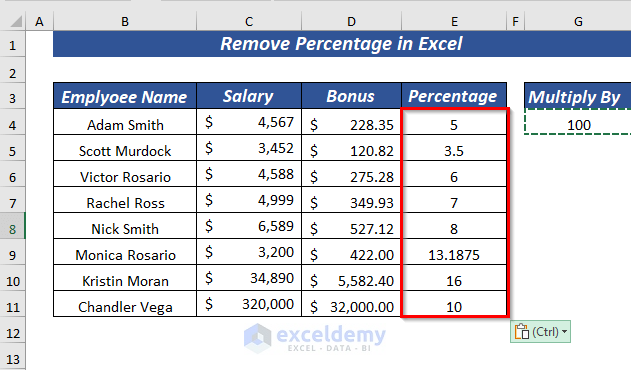
This will remove the Percentage sign but the value will remain the same.
Method 4 – Remove Percentage Using Custom Format
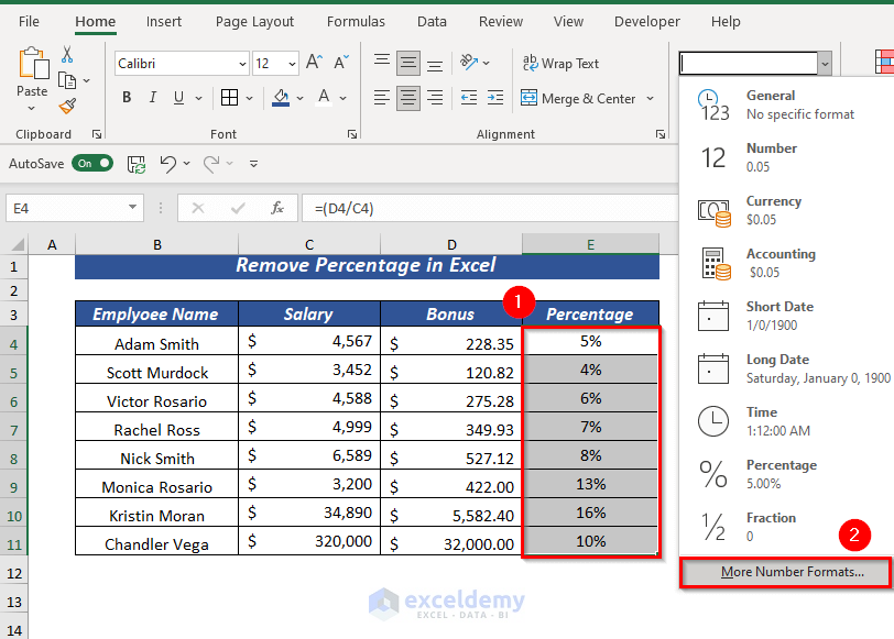
Select the cell or cell range from where you want to remove the percentage sign while keeping the value.
Open the Home tab >> from Number Format >> select More Number Formats
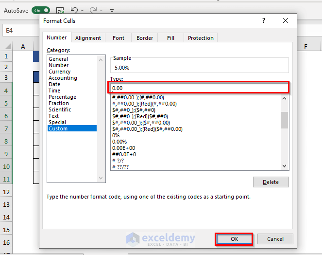
⏩ Select Custom.
Select 0.00% as the Type.
Place the cursor before the percentage and press CTRL + J.
CTRL + J will create a new line.
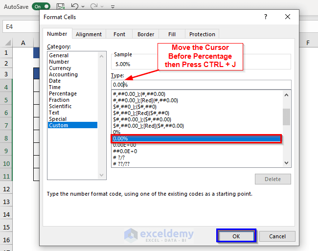
The percentage will be removed from Type. Click OK.
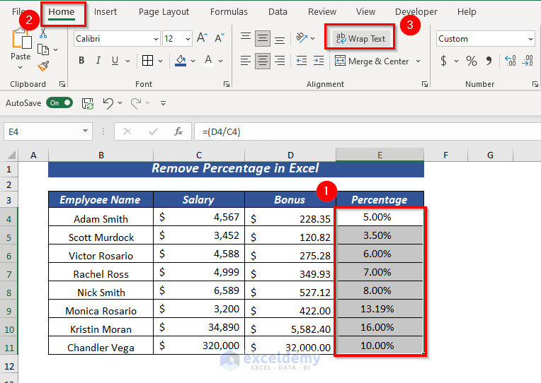
Select the cell range to apply Wrap Text.
Open the Home tab >> from Alignment >> select Wrap Text
Wrap Text will be applied to the selected cells.
To hide the line where the percentage is.
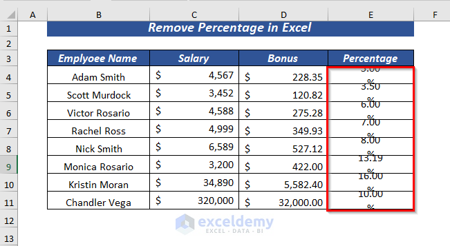
Decrease the Row Height.
Select the cell or cell range from where you want to remove the percentage sign.
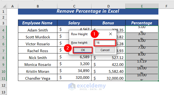
Open the Home tab >> go to Cells >> from Format >> select Row Height
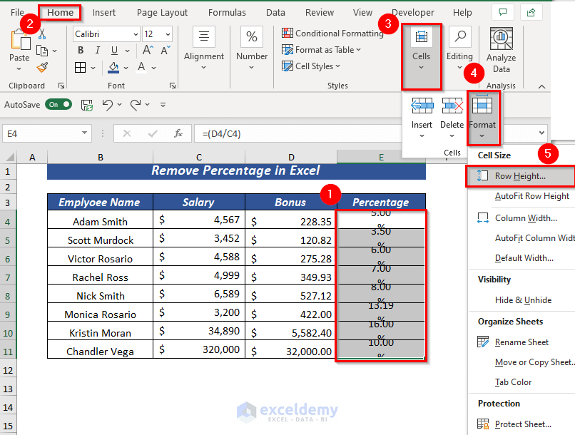
➤ Enter the row height as 16.
Click OK.
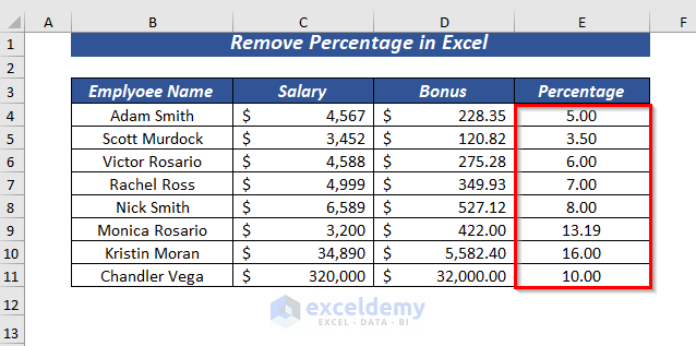
It will hide the percentage sign only the values will be visible.
Method 5 – Using Power Query to Remove Percentage in Excel
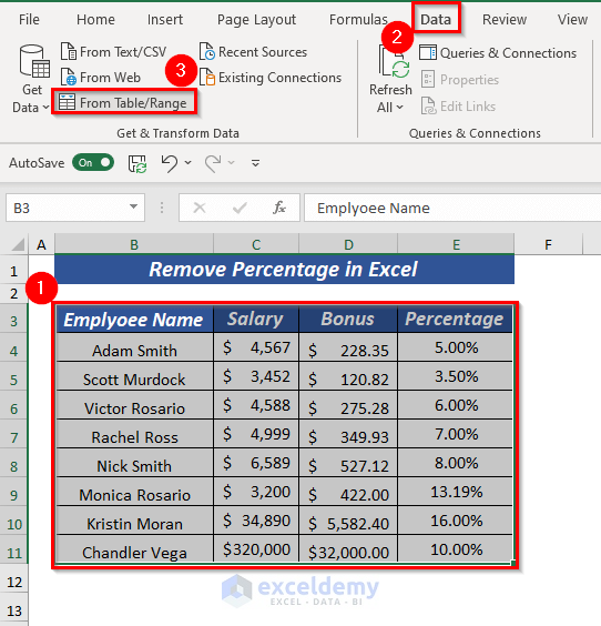
Select the cell range.
Open the Data tab >> select From Table/Range
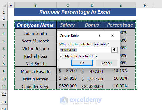
➤ Checkmark on My table has headers.
Click OK.
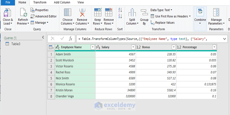
A new window will be displayed.
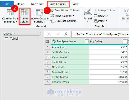
From Add Column tab >> select Custom Column.
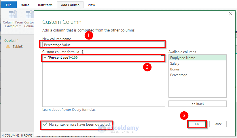
A Custom Column dialog box will pop up.
⏩ In the New column name, select Percentage Value.
⏩ In the Custom column formula, select [ Percentage ]*100.
Click OK.
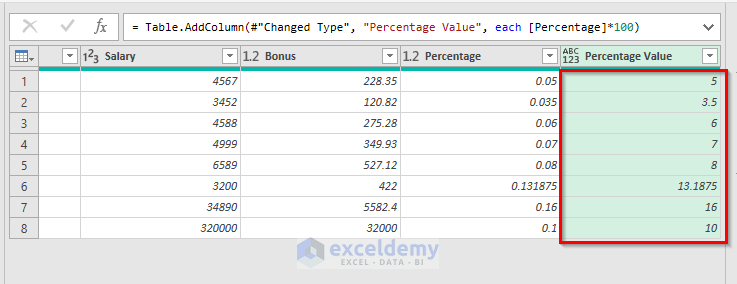
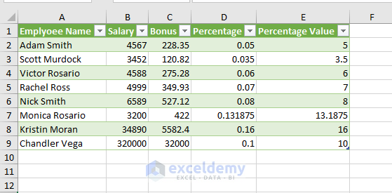
It will add a new column named Percentage Value showing the values.
In case you want to load the table in the worksheet.
Open Home tab >> from Close & Load >> select Close & Load To…
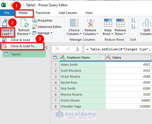
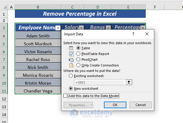
A dialog box will pop up. You can choose the option to place the data.
⏩ Select New worksheet.
Click OK.
It will import the data into a new worksheet.
Download Practice Workbook
Related Articles
- How to Calculate Total Percentage from Multiple Percentages in Excel
- How to Calculate Percentage of Month in Excel
- How to Calculate Percentage of Percentage in Excel
- How to Calculate Percentage Based on Conditional Formatting
- How to Calculate Percentage in Excel Based on Cell Color
- Percentage Showing as Thousand in Excel
- Why Are My Percentages Wrong in Excel?
- How to Find the Percentage of Two Numbers in Excel
- How to Calculate Percentage Complete Based on Dates in Excel
- How to Calculate Error Percentage in Excel
- How to Calculate Cumulative Percentage in Excel
<<Go Back to Calculating Percentages in Excel | How to Calculate in Excel | Learn Excel
Get FREE Advanced Excel Exercises with Solutions!

