Method 1 – Change Format as General to Remove Percentage Without Changing Values
STEPS:
- Insert a new column to compare. After removing the percentage symbol, the values will remain the same.
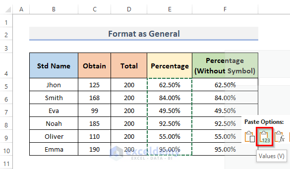
- Copy the entries from the Percentage column to the Percentage (Without Symbol) column. Use the paste option as Value; this will copy the percentage with the formula; we use the C5/D5 formula in the Percentage column.
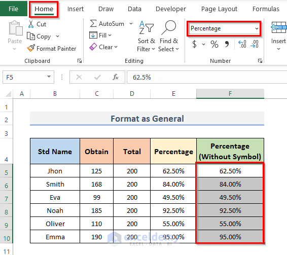
- Select the cell range F5:F10 from the new column F and go to the Home tab from the ribbon. In the Number category, you can see that this will be formatted as a Percentage.
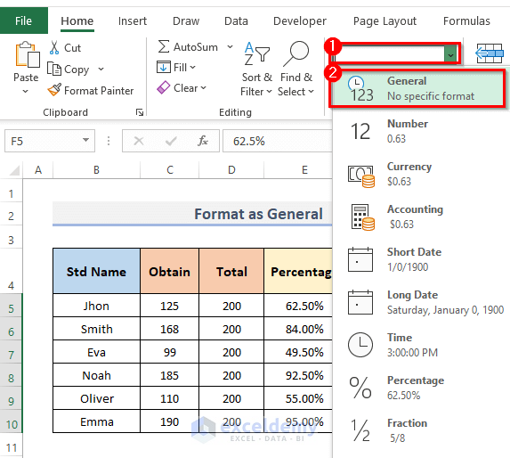
- To change the format, click on the drop-down menu. Select General.
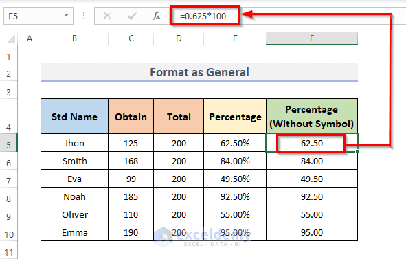
- You can see the cell ranges are now displaying the value without the percentage symbol.
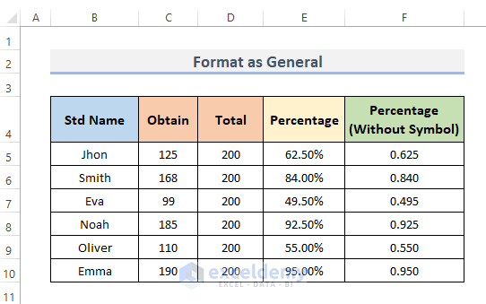
- To keep the value as same as column E, multiply each data by 100 to place the value without changing and eliminate the percentage symbol.
Method 2 – Apply Number Formatting for Removing Percentage in Excel
STEPS:
- Add a new column for comparison. After deleting the % sign, the numbers will remain the same.
- Copy the Percentage column’s contents to the Percentage (Without Symbol) column. Use the paste option as Value; because we are using the C5/D5 formula in the % column, this would copy the percentage with the formula.
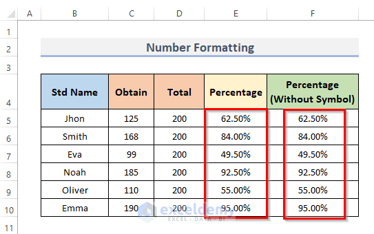
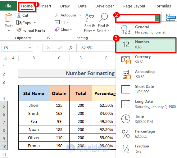
- Go to the Home tab on the ribbon. When you pick the cell range F5:F10 from the new column F, this is formatted as Percentage, as you can see in the Number category.
- Click the drop-down menu again to alter the format. Go to Number.
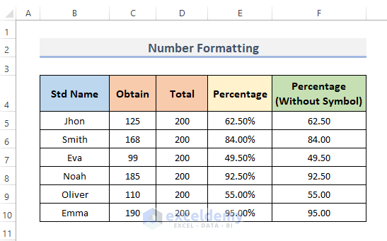
- The value is now shown without the percentage indicator in the cell ranges.
- The values are not the same. Multiply each of the data by 100 to position the value without changing it and remove the percentage symbol to retain the value the same as column E.
Method 3 – Utilize Format Cells to Omit Percentage Without Changing Values
STEPS:
- The first technique adds a new column for comparison. The figures will remain the same after removing the percent indication. Transfer the contents of the Percentage column to the Percentage (Without Symbol) column.
- Use the paste option as a value instead of copying the percentage with the formula because we are utilizing the C5/D5 formula in the percentage column.
- Select the new column and go to the Home tab from the ribbon.
- Click on the tiny icon, under the Number category to open the Format Cells dialog.
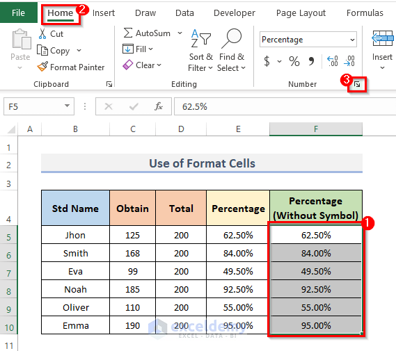
- You can just select the cell range and right-click on your mouse, click on the Format Cells.
- Use the keyboard shortcut Ctrl + 1 to display the Format Cells window.
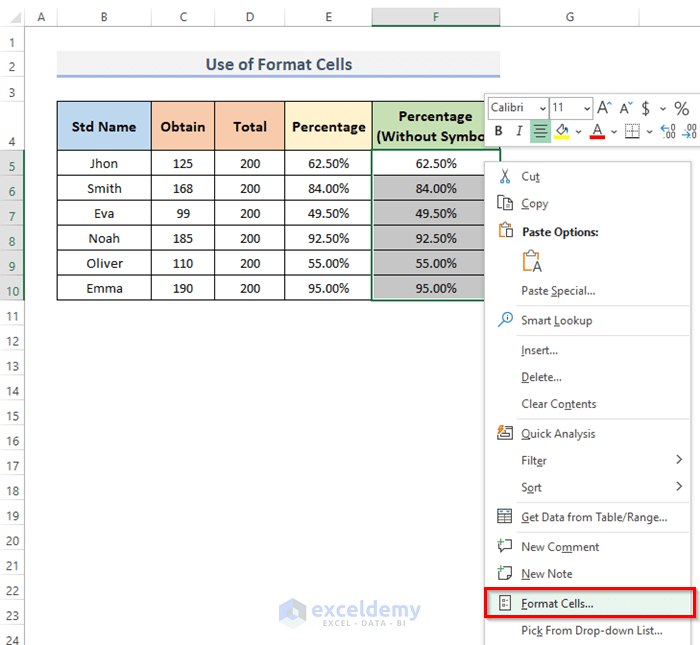
- Use any of those approaches to open the Format Cells dialog box.
- Go to the Number menu and click on Custom.
- Type field, you will notice that 0.00% formatting has already been provided.
- Place the cursor immediately before the percent symbol in the Type field, and press Ctrl + J.
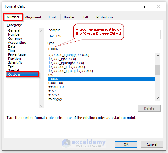
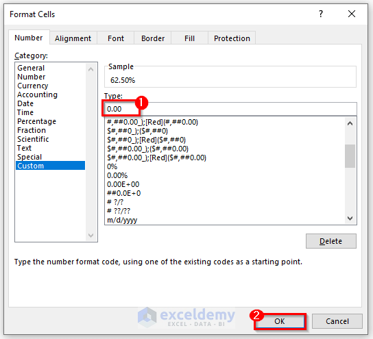
- You will note that the formatting in the Type field is now altered to 0.00 only, omitting the percentage sign.
- Press the OK button to close the Format Cells dialog box.
- You will notice that the % symbols are still there in the figures.
- Click Wrap Text from the Home tab and choose the range of cells F5:F10.
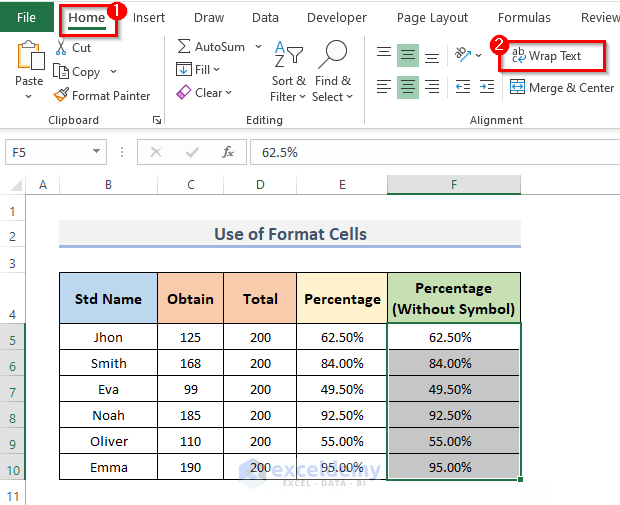
- You will see that the percentage sign is absent from cells F5 through F10.

Method 4 – Multiply Specific Number for Removing Percentage Symbol
STEPS:
- Select the whole range F5:F10 and go to the Home tab to change the format to Number.
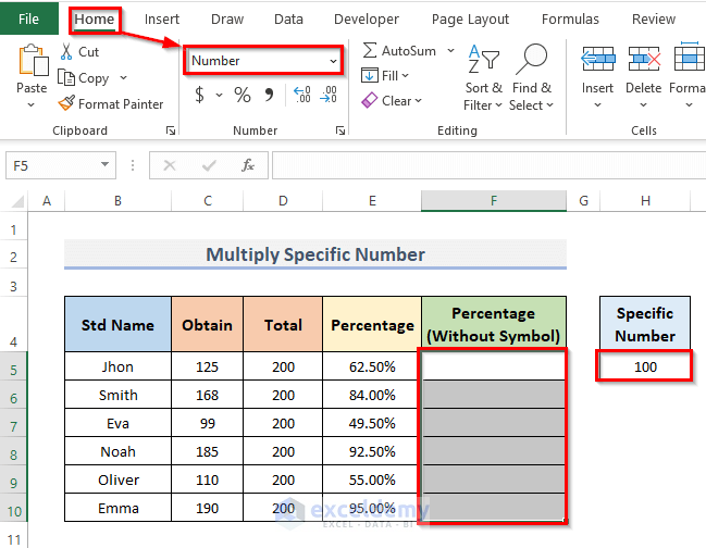
- Insert the formula in cell F5.
=E5*$H$5- Press Enter.
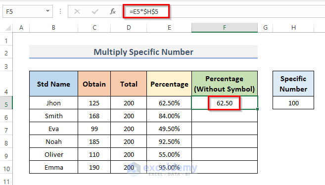
- Drag the Fill Handle down or double-click on the plus (+) icon.
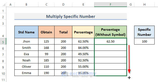
- See the percentage symbol is now removed and the value still remains the same.
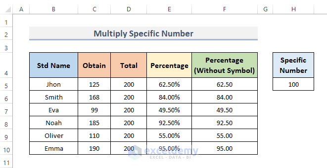
Note: Use the dollar $ sign cause we want the cell as an absolute reference. As we don’t want to change the cell. While using the absolute reference, the cell will remain the same if you duplicate the formula anywhere else.
Method 5 – Remove Percentage with Excel Paste Special Feature
STEPS:
- Copy the cell G5.
- Select the cell range E5:E10.
- Right-click on the mouse and select Paste Special.
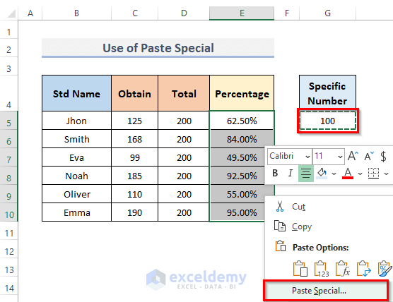
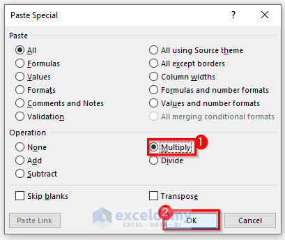
- This will display the Paste Special dialog box.
- In the Operation section, select Multiply.
- Click on the OK button to close the dialog box.
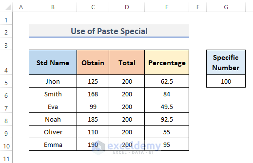
- You can now see the percentage symbol removed, and the values remain unchanged.
Method 6 – Use Excel Formula to Take Off Percentage in Excel
STEPS:
- Choose the cell where you want to remove the percentage symbol without changing the values. Select cell F5.
- Enter the following formula there.
=VALUE(LEFT(TEXT(E5,"00.00%"),5))- To complete the operation hit the Enter key.
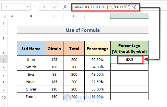
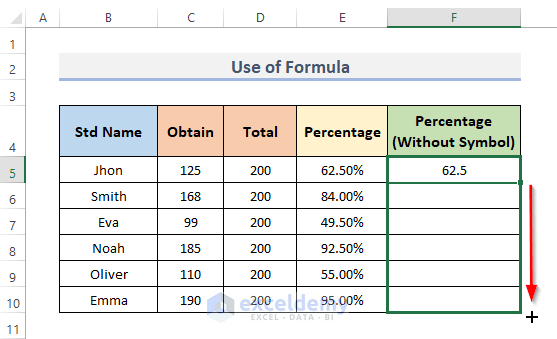
- Replicate the formula throughout the range, and drag the Fill Handle downward. To auto-fill the range, double-click on the plus (+) symbol.
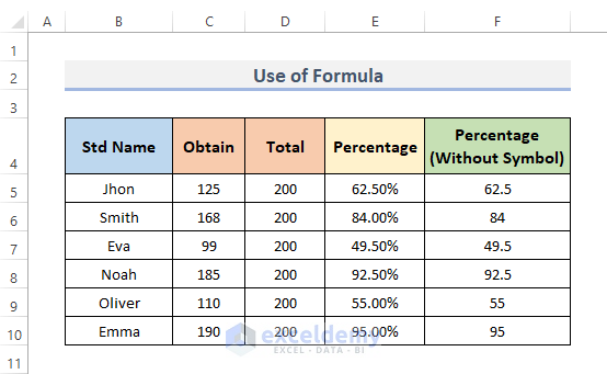
- Get the result.
How Does the Formula Work?
- TEXT(E5,”00.00%”): This function accepts the content of cell E5 as an argument and outputs a text string in the format 00.00.
- LEFT(TEXT(E5,”00.00%”),5): The 5 characters on the left side of the strings returned by the TEXT function will be extracted with this method.
- VALUE(LEFT(TEXT(E5,”00.00%”),5)): This returns the number from the left function’s string format.
Note: The arguments inside the functions should be cautiously entered in this formula. The rounding value, which is 2 in this case, is represented using the format 00.00. You must specify a rounding value that is appropriate for your needs.
Method 7 – Excel VBA Macro to Remove Percentage Symbol Without Changing Values
STEPS:
- Go to the Developer tab from the ribbon.
- From the Code category, click on Visual Basic to open the Visual Basic Editor. Or press Alt + F11 to open the Visual Basic Editor.
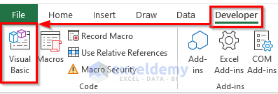
- This will appear in the Visual Basic Editor where we write our code to create a table from a range.
- Click on Module from the Insert drop-down menu bar.
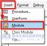
- This will create a Module in your workbook.
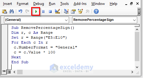
- Copy and paste the VBA code shown below.
VBA Code:
Sub RemovePercentageSign()
Dim r, c As Range
Set r = Range("E5:E10")
For Each c In r
    c.NumberFormat = "General"
    c = c.Value * 100
Next
End Sub- Run the code by clicking the Run Sub button or pressing the keyboard shortcut F5.
- Remove the percentage symbol without changing the values.
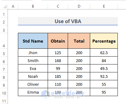
Note: While using VBA Macros, save your file as a macro-enabled file. And the extension for the file will be .xlsm.
Method 8 – Apply Power Query to Remove Percentage Symbol in Excel
STEPS:
- Go to the Data tab from the ribbon.
- From Get & Transform Data click From Table/Range.
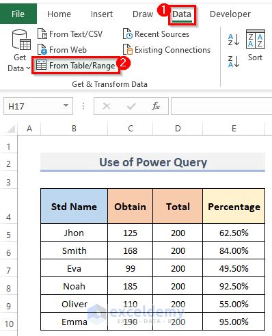
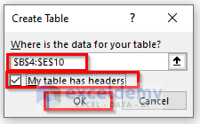
- A Create Table dialog box will appear.
- In Where is the data for your table?, select the range $B$4:$E$10. Tick My table has headers, to let Excel know that the first row of your table is the header.
- Click OK.
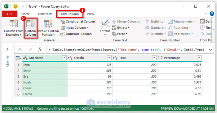
- This will open the Power Query Editor.
- Go to Add Column from the menu bar.
- Under General Group, click on Custom Column.
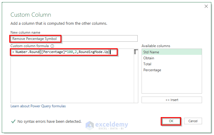
- The Custom Column window will display, set the New column name; Remove Percentage Symbol.
- In the Custom column formula field, enter the following formula.
=Number.Round([Percentage]*100,2,RoundingMode.Up)- Click the OK button to finish the process.
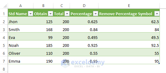
- This will add a new column without changing the values. The new column contains all the numbers from the Percentage column but without the percentage symbol.

- Close the Power Query Editor, closing it a window will appear asking Do you want to keep your changes?. Click on Keep.

- The table from the power query will now be structured with percentage values on the worksheet.
Download Practice Workbook
You can download the workbook and practice with them.
Related Articles
- How to Remove Currency Symbol in Excel
- How to Remove Dollar Sign in Excel
- How to Remove Pound Sign in Excel
- How to Remove Plus Sign in Excel
- How to Remove Negative Sign in Excel
<< Go Back to Remove Symbol in Excel | Excel Symbols | Learn Excel
Get FREE Advanced Excel Exercises with Solutions!

