How to Remove Signs from Numbers in Excel – 6 Methods

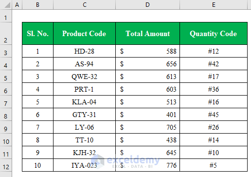
The sample dataset showcases total Sales Amount, Product Code, and Quantity Code. There are unwanted signs in the Quantity Code column.

Method 1 – Using the Find & Replace Feature to Remove Signs from Numbers

Steps:

• Press Ctrl+H to open the “Find and Replace” window.

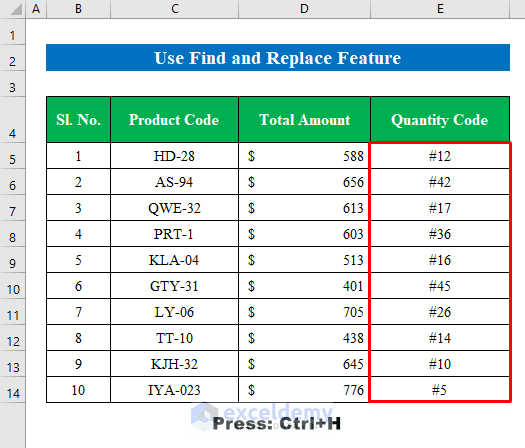
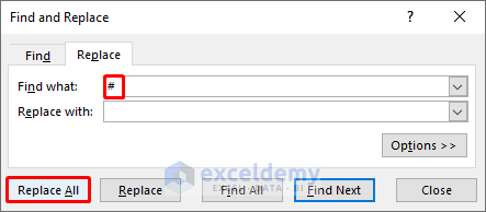
• Enter the hash mark(#) in “Find what”.
• Click “Replace All”.

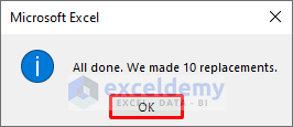
• A confirmation window will be displayed. Click OK.

This is the output.

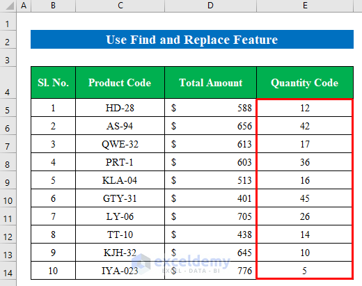
Note: If you have different types of signs, enter the sign in “Find what” to remove it.

Read More: How to Remove Pound Sign in Excel

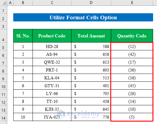
Method 2 – Utilizing the Format Cells Option to Remove Signs from Numbers

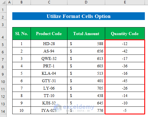
To remove the dash sign (–) in column E:

Steps:

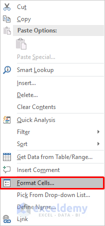
• Select E5:E14 and right-click.

• Choose “Format cells”.

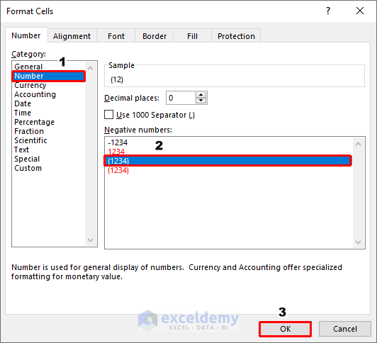
• In the new window, select “Number” and choose a format.
• Click OK.

This is the output.

Read More: How to Remove Currency Symbol in Excel

Method 3 – Using the SUBSTITUTE Function to Remove Signs from Numbers

3.1 Remove a Single Sign

Steps:

• Choose a cell. Here, G5.
• Enter the formula in the cell:

The SUBSTITUTE function will find a sign or string and replace it with another string.

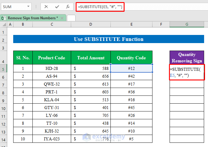
• Press Enter  button to see the result.
• Drag down the Fill Handle to see the result in the rest of the cells.

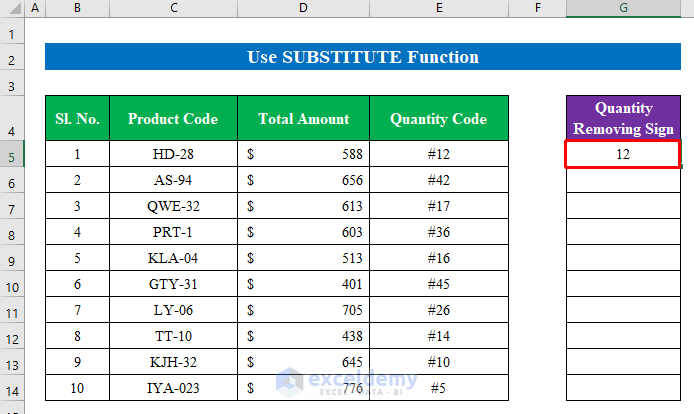
This is the output.

3.2 Remove Multiple signs

There are different signs at the beginning and in the middle of numbers in the Quantity Code column.

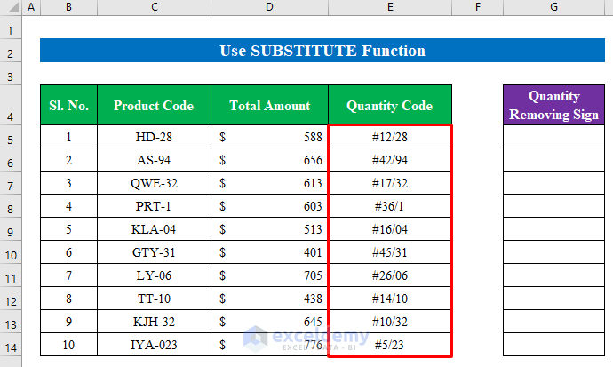
Steps:

• Choose a cell, here G5.
• Enter the formula:

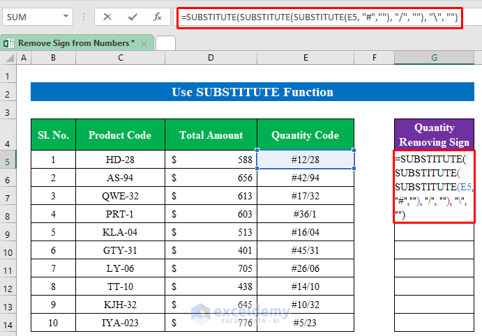
• Press Enter to see the result.
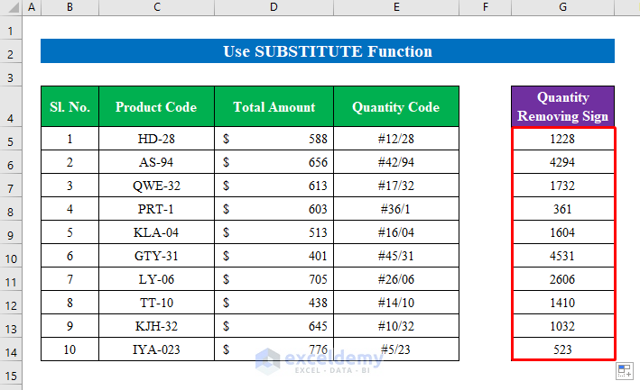
• Drag down the Fill Handle to see the result in the rest of the cells.

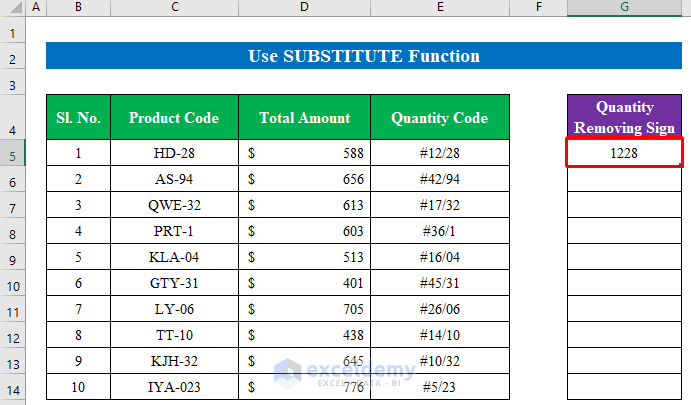
This is the output.

Read More: How to Remove Plus Sign in Excel

Method 4 – Using the Flash Fill Feature to Remove Signs from Numbers

Steps:

• Create a new column.
• Enter at least two numbers from the list to enable the fill handle.

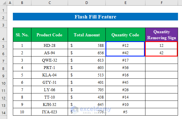
• Selecting both cells drag down to fill Handle.
• Click the “Fill” icon and choose “Flash Fill” option.

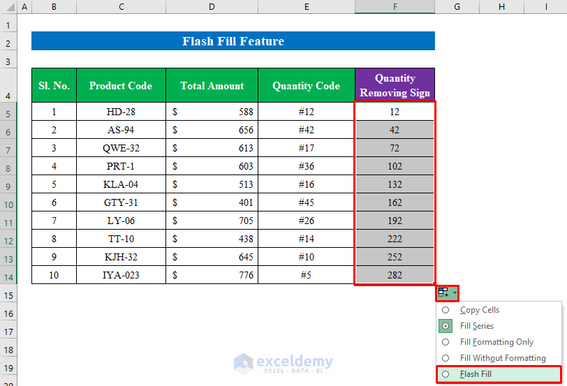
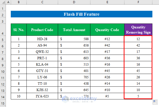
This is the output.

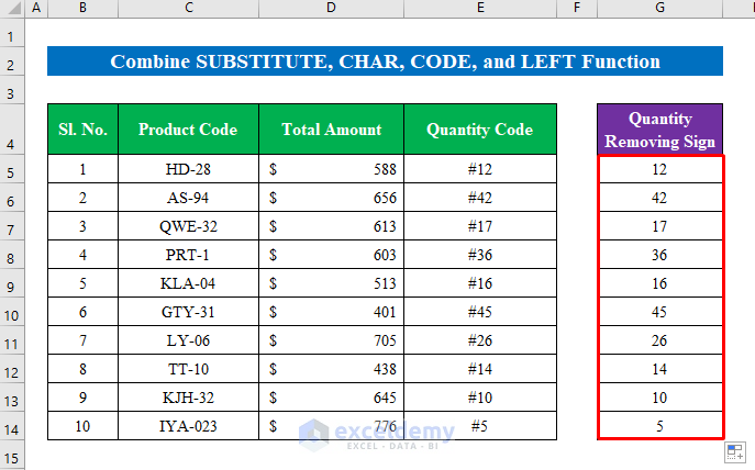
Method 5 – Combining the SUBSTITUTE, CHAR, CODE, and LEFT Functions to Remove Signs from Numbers

Steps:

• Choose a cell, here G5.
• Enter the formula:

• The LEFT function will extract numbers from the selected cell (E5).
• The CODE function will return a numeric code from the given string.
• The CHAR function identifies characters based on the number.
• The SUBSTITUTE function will find a sign or string and replace it with another string.

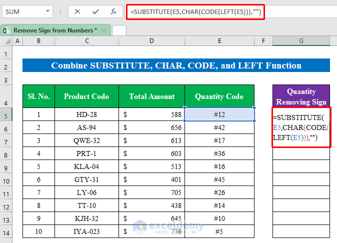
• Press Enter to see the result.
• Drag down the Fill Handle to see the result in the rest of the cells.

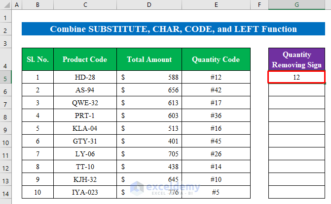
This is the output.

Method 6 – Merge the RIGHT and LEN Functions to Remove Signs from Numbers in Excel

Steps:

• Choose a cell, here G5.
• Enter the formula:

• The LEN function returns the length of a given string.
• The RIGHT function extracts a given number of characters from the right side of a string. Here (E5)-1 removes one character from the right side.

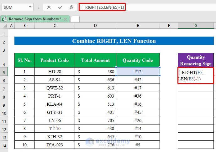
• Press Enter to see the result.
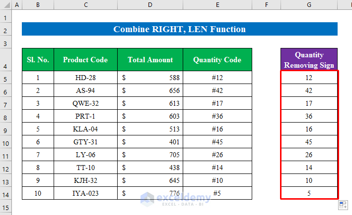
• Drag down the Fill Handle to see the result in the rest of the cells.

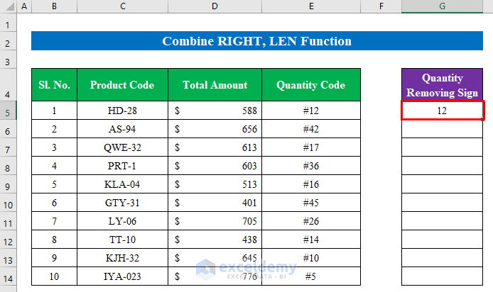
This is the output.

Things to Remember

• To remove the minus sign (–), use the ABS() formula. In the bracket portion enter the cell number.
• You can also use the VALUE function to delete the dollar sign($). It must be on the right side of the numbers.

Download Practice Workbook

Download the practice workbook.

Related Articles

• How to Remove Dollar Sign in Excel
• How to Remove Dollar Sign in Excel Formula
  
• How to Remove Negative Sign in Excel
• How to Remove Percentage Symbol in Excel
• How to Remove Percentage Symbol in Excel Without Changing Values

<< Go Back to Remove Symbol in Excel | Excel Symbols | Learn Excel