How to Remove Sort by Color in Excel (With Easy Steps)

Step 1 – Add an Extra ‘Index’ Column

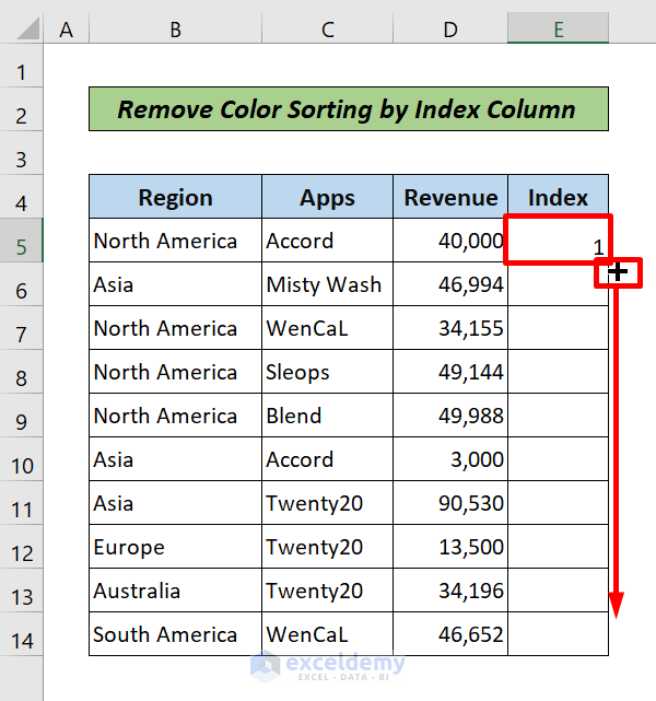
• Enter a 1 in a blank cell of the Index column to the right of the data set.
• Drag the Fill Handle to the remaining cells of the column.

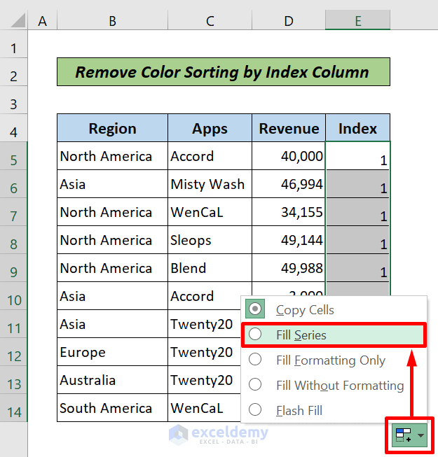
• Select Fill Series from the Autofill Option.

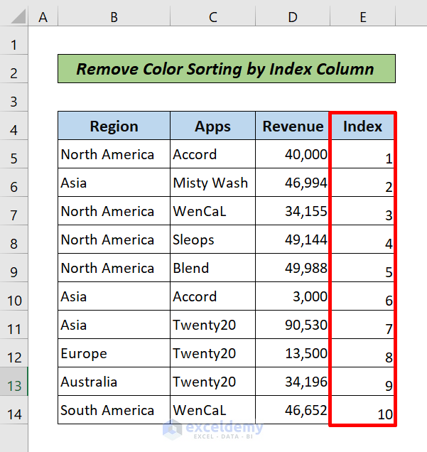
Here is the Index Column,

Step 2 – Sort Data by Color

• Select the entire table> go to the Data tab> the Sort & Filter group > Click on the Sort

• A Sort window will pop up. Mark the My data has headers checkbox at the top-right corner.
• To Sort by, click the drop-down arrow and select the column header (In this case, Revenue) that you want to sort by the colors of the cells of that column. For Sort on values, select Cell Colors and for Order, select your first cell color Red. Keep the Order value as On Top.

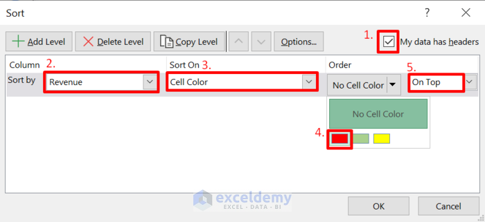
• Click on Add level in the top-left to add your other color levels.

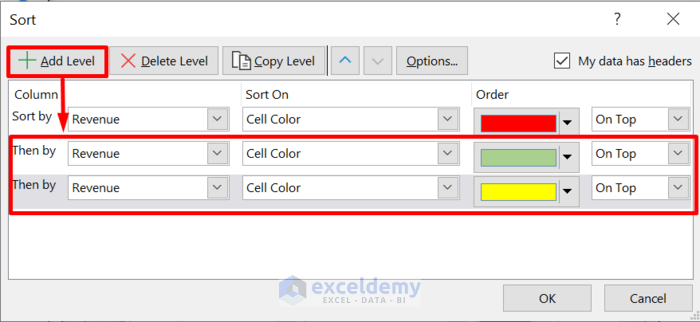
• Click OK and Excel will sort the dataset by color.

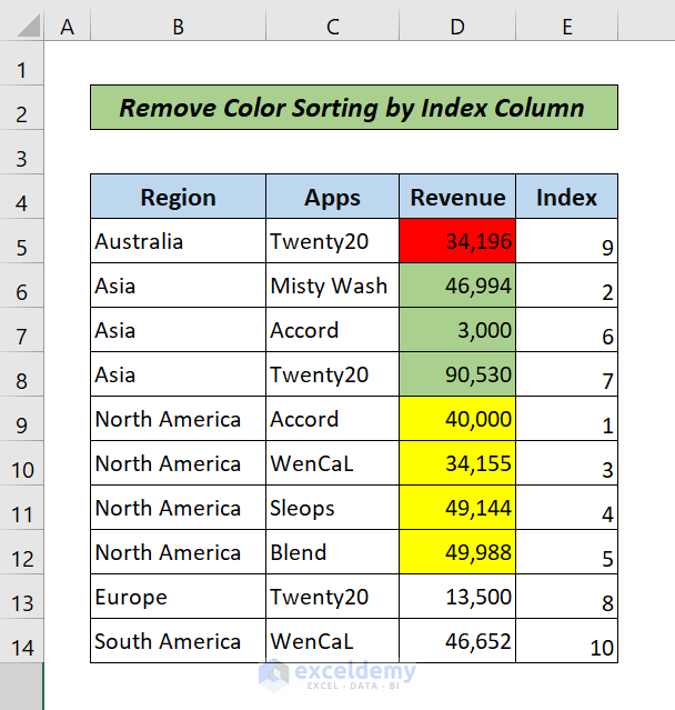
Step 3 – Remove Sort

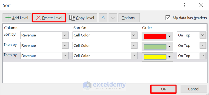
• Select the entire table > Go to the Data tab > From the Sort & Filter group, click on the Sort A Sort window will pop up.
• Delete the previous levels. Press OK.

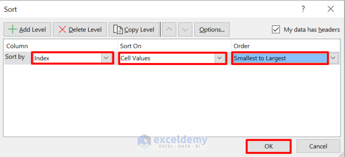
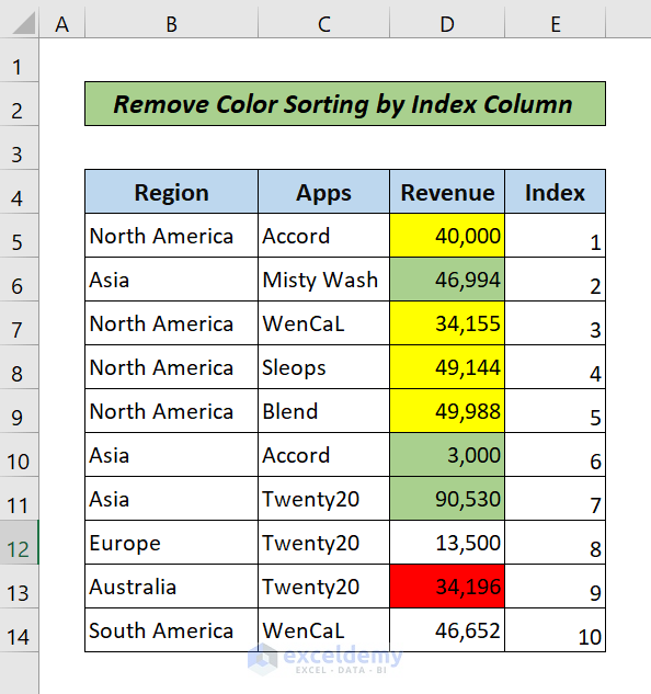
• Select the entire table. Go to Data tab> Sort. Under the Sort window, select Index, Cell values and Smaller to Largest for the Column, Sort On and Order box respectively. Click Ok.

Here is the restored previous sorting dataset,

Read More: How to Undo Sort in Excel

Download Practice Book

<< Go Back to Remove Sort | Sort in Excel | Learn Excel