Dataset Overview
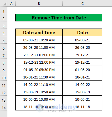
We have a dataset that contains information about several dates and times in Column B. We will remove time from the date of our Pivot Table step-by-step methods. Here’s an overview of the dataset.
Step 1 – Create a Pivot Table
- Open your Excel workbook.
- Select the dataset that contains dates and times in Column B.
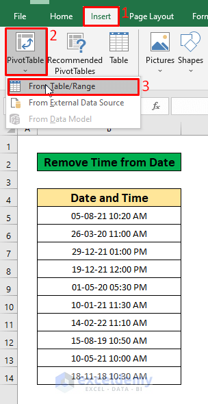
- Go to the Insert tab on the ribbon.
- Click on PivotTable and choose From Table/Range.
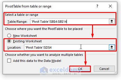
- In the PivotTable from table or range dialog, select cells B4:B14 as the data range.
- Check the Existing Worksheet option and click OK.
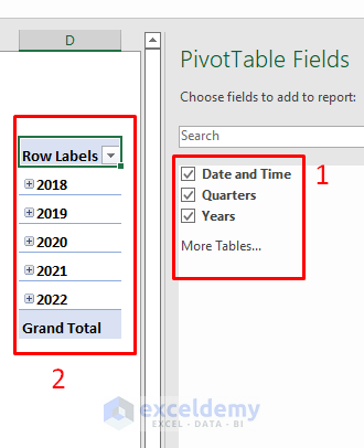
You’ll now have a PivotTable with the Date and Time, Quarters, and Years fields grouped.
Step 2 – Remove Time from Date
- Select the PivotTable data (e.g., cells D4:D15).
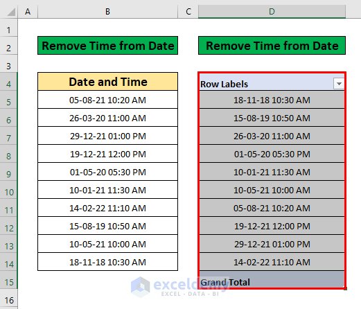
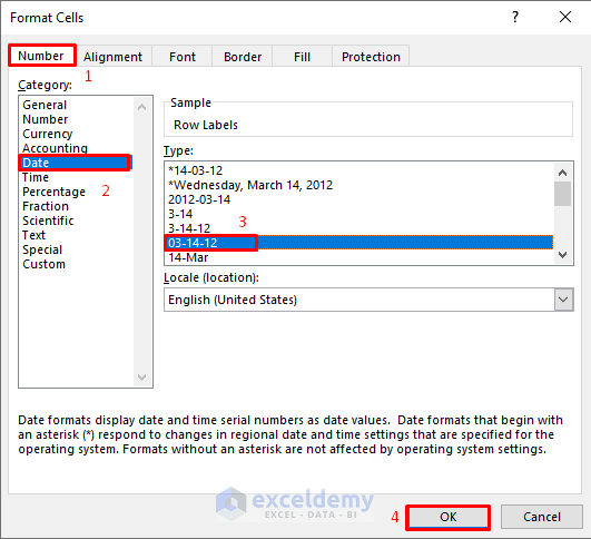
- Press Ctrl + 1 on your keyboard to open the Format Cells dialog.
- In the dialog, choose the Number category.
- Select Date from the options.
- Under Type, choose the format 03-14-12.
- Click OK.
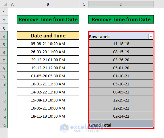
Your PivotTable will now display dates without the time component.
Read More: How to Change Date Format in Pivot Table in Excel
Things to Remember
To access the Format Cells dialog, press Ctrl + 1 on your keyboard.
Download Practice Workbook
You can download the practice workbook from here:
<< Go Back to Pivot Table Date Format | Pivot Table Formatting | Pivot Table in Excel | Learn Excel
Get FREE Advanced Excel Exercises with Solutions!


I have changed the format of DateTimeColumn from the Format Cells in a pivot table but it did not work.
Hi HASNAIN AHMAD,
Thank you very much for following our article. You mentioned that even after changing the format of the Date_Time column, it did not work properly. To understand your problem, we follow the full process again and found everything is working properly. We suggest you read the steps again and apply them carefully. Hope you will get the desired result.