[Fixed] Report Connections Slicer Not Showing All Pivot Tables

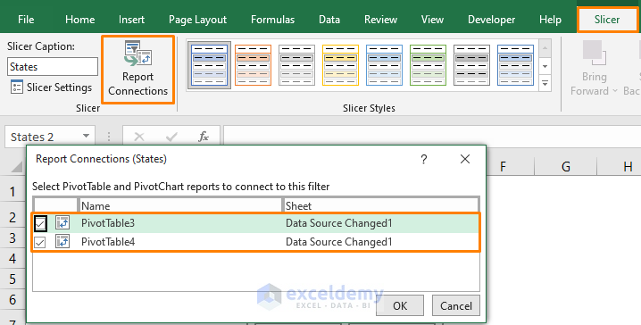
Report Connections is a feature to manage Pivot Tables that are connected with the Slicer tool.

This feature will work if you add Slicer to a Pivot Table or several Pivot Tables. And, you can connect or disconnect those Pivot Tables to filter together using the Slicer.

In the below screenshot, the check box before the Pivot Table name is used to connect to the tool.

Issues and Solutions for Report Connections Slicer Not Showing All Pivot Tables

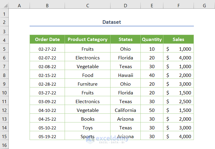
In the sample dataset Product Category is given with their Order Date, Quantity, and Sales based on the States of the U.S.

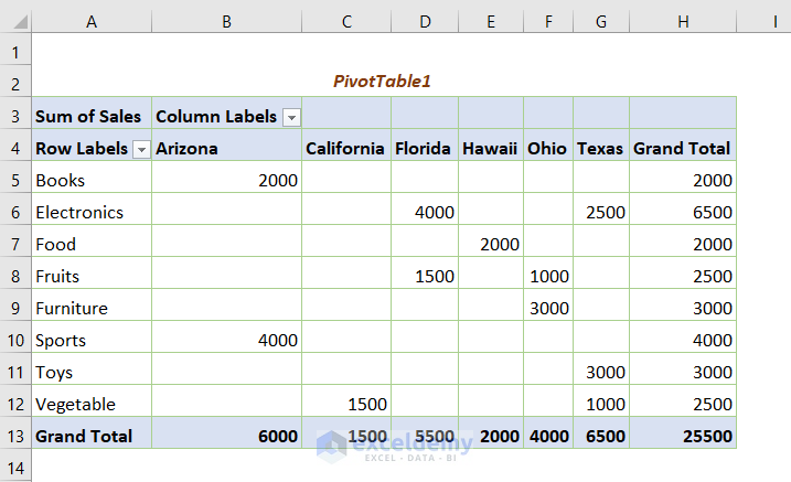
• Create a Pivot Table for the above dataset.
• Go to Insert tab > Pivot Table > From Table/Range.

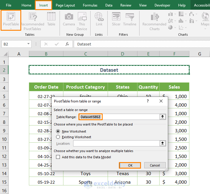
• Press OK.

Problem 1 – When No Connections Are Found

Excel reports No connections found as below.

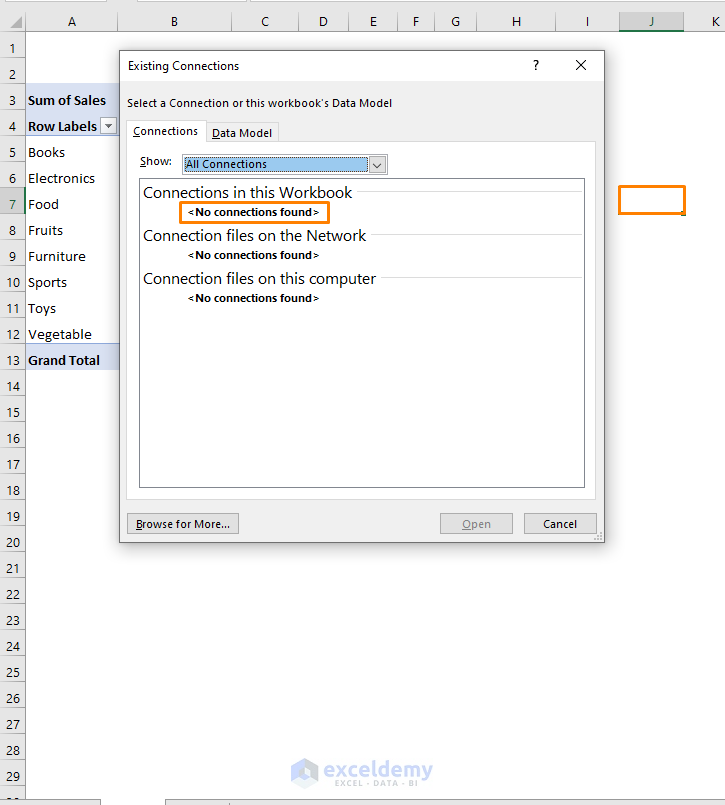
I tried the Slicer while selecting the blank J7 cell outside the Pivot Table. That’s why Excel returned aNo connections found.

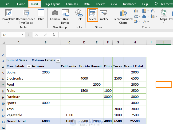
The Solution to the Issue

• Insert the Slicer tool while putting the cursor over a cell within the Pivot Table. 

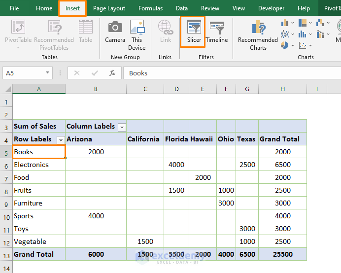
• The filtering options (in the Insert Slicers dialog box) will appear.
• Check the box before the States option.

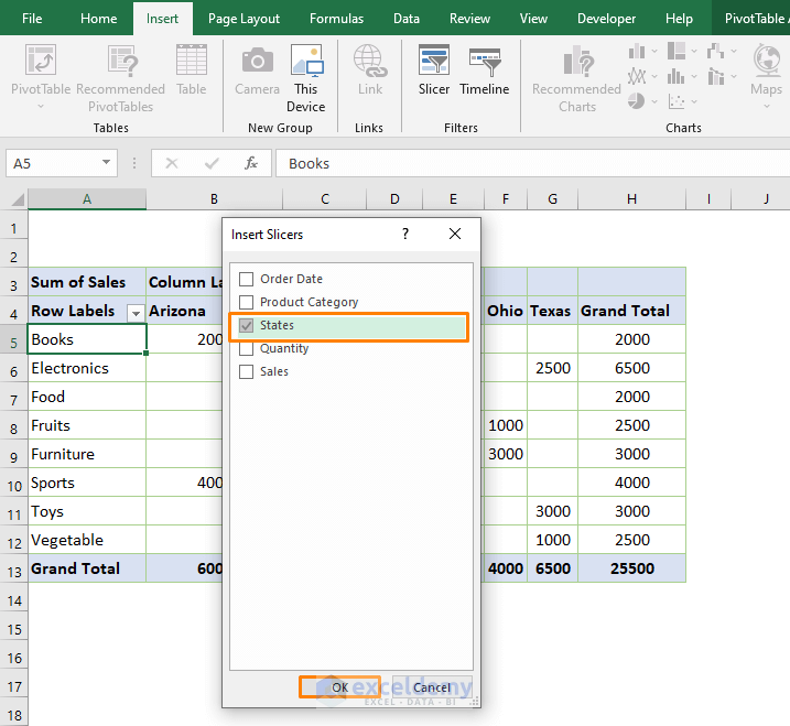
• Press OK, and all States will be available to filter.

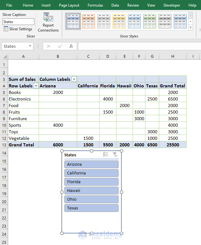
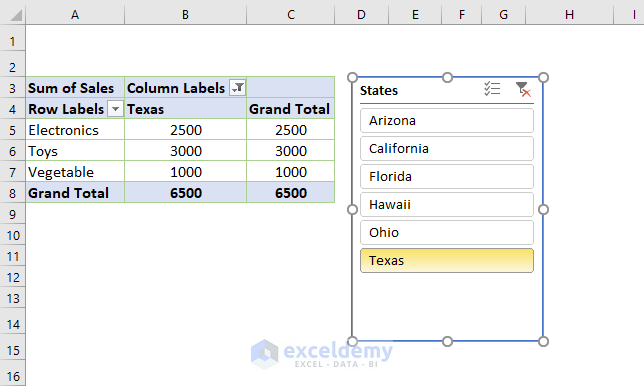
• Click on any state among the options (e.g. Texas), and the Slicer will work properly.

Read More: How to Format Slicer in Excel

Problem 2 – If Slicer Is Not Connected with All Pivot Tables

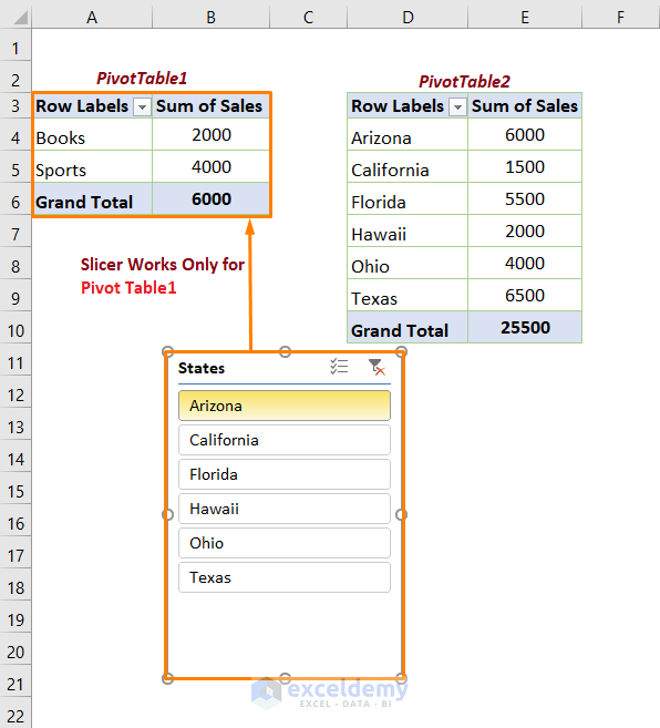
In the following figure where two Pivot Tables (PivotTable1 and PivotTable2) are available but the Slicer doesn’t work for PivotTable2.

• Click on the Report Connections feature.

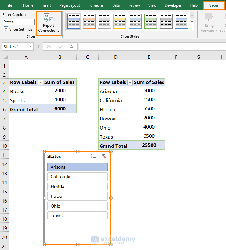
• The PivotTable2 is not connected. That’s the main issue.

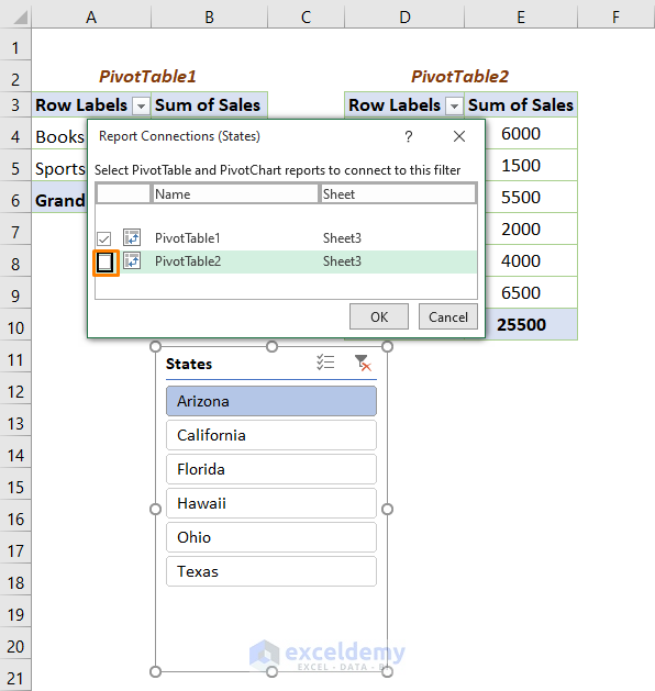
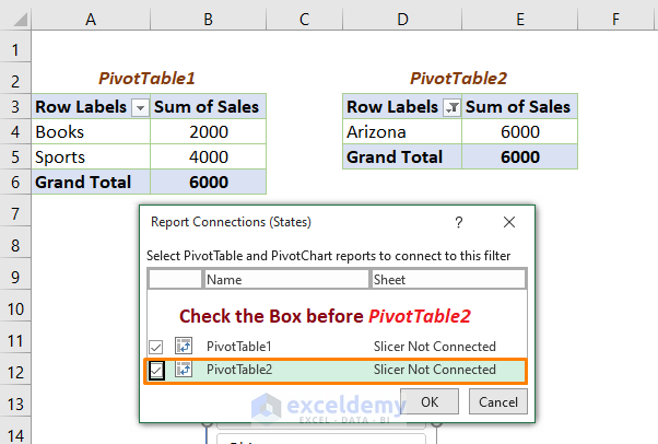
The Solution to the Issue

Check the box before the PivotTable2.

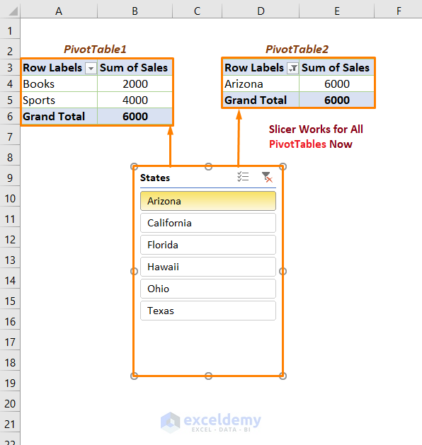
The Slicer is working for the two Pivot Tables simultaneously.

Problem 3 – When Source Data Range Is Changed

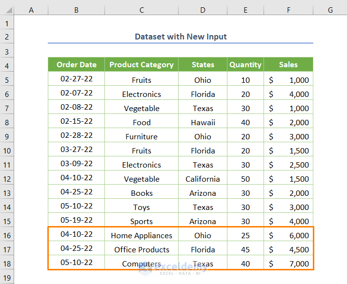
The B16:F18 cells are to be added to the existing Pivot Table.

Right-click (while selecting a cell within the Pivot Table) and pick the Refresh option.

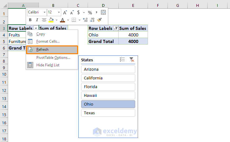
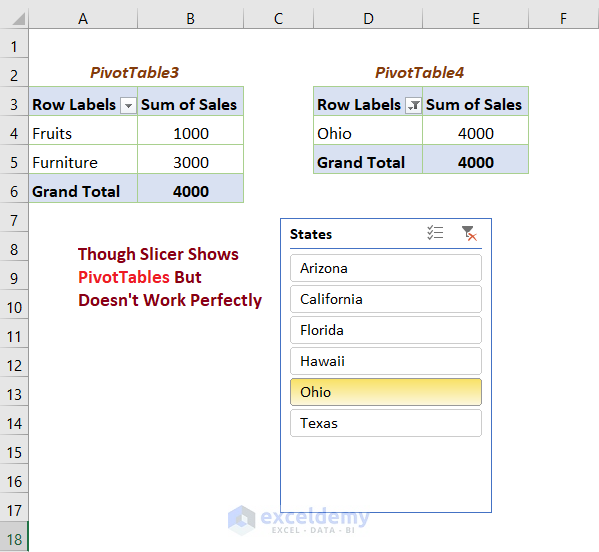
The Slicer shows PivotTables without all the relevant data. That means the PivotTables are not updated with the new data.

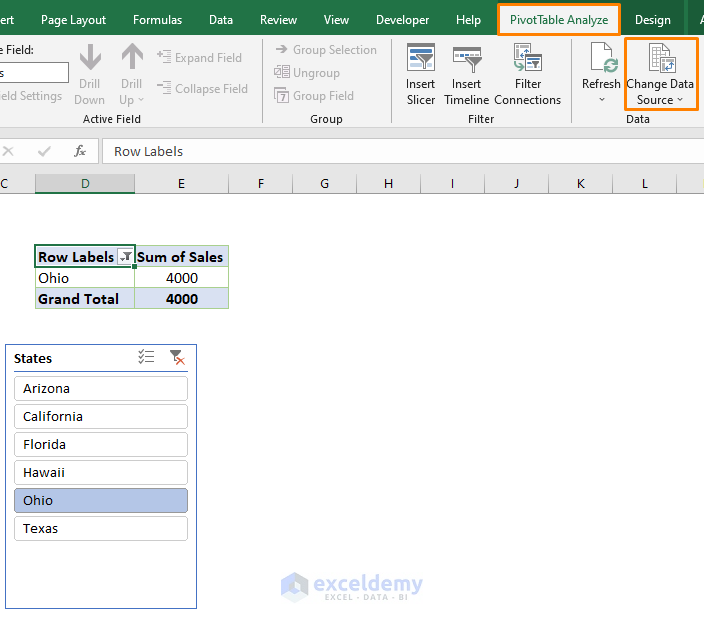
• Click on the Change Data Source from the PivotTable Analyze tab.

• Specify the source of data (e.g. $B$4:$F$18).

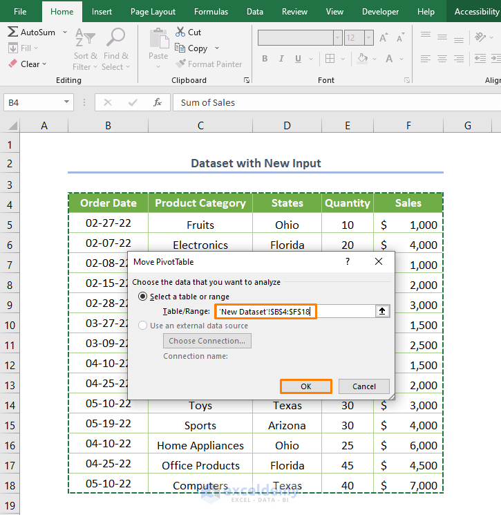
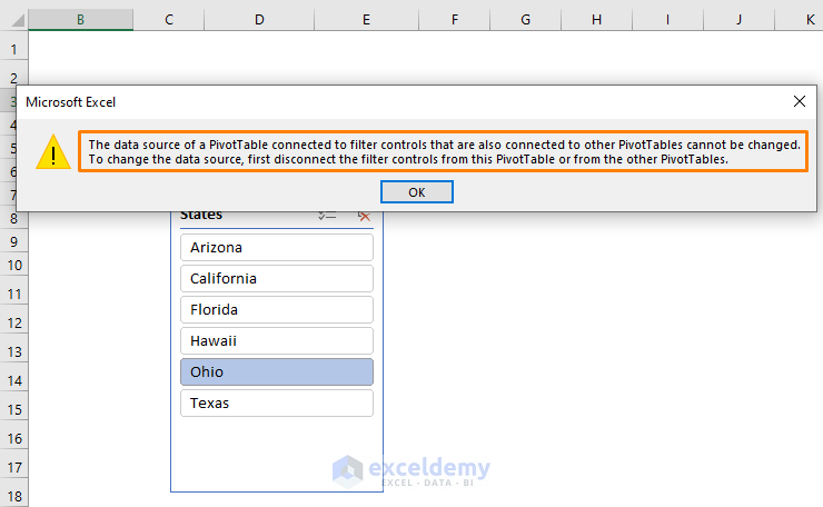
A message states that you cannot change the source of the dataset until you remove the filter controls (Slicer).

The Way of Fixing the Issue:

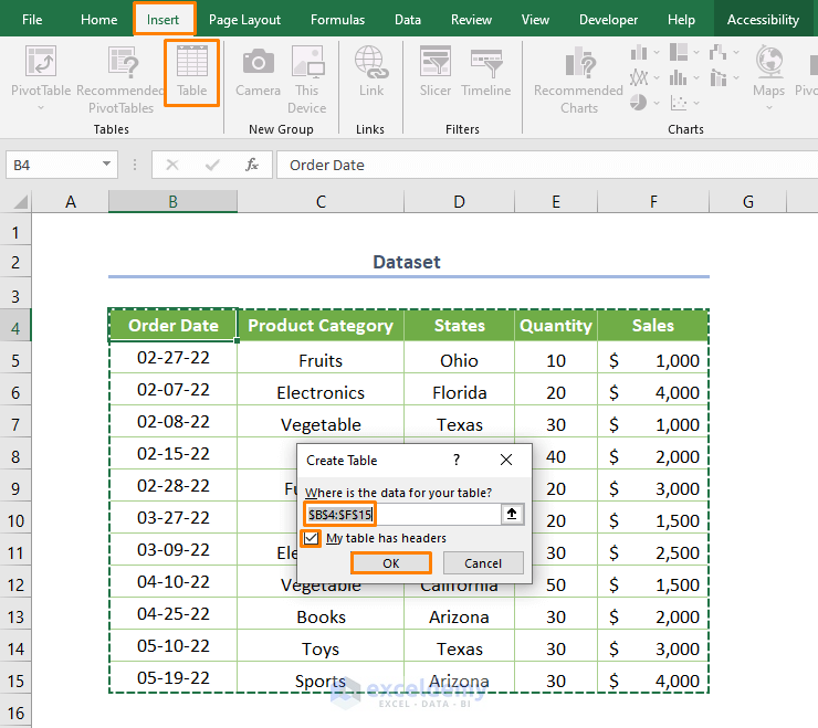
• Create a table from the Insert tab > Table option (or press CTRL + T) while selecting a cell within the dataset.

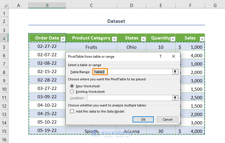
• Create the Pivot Tables by using Table2.

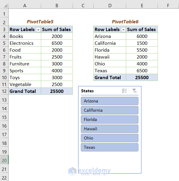
• Add the Slicer (also check the Report Connections where you need to connect two Pivot Tables).
• Thee following output will be returned.

• Add the new input (B16:F18 cells) to Table2.
• Right-click and choose the Refresh option.

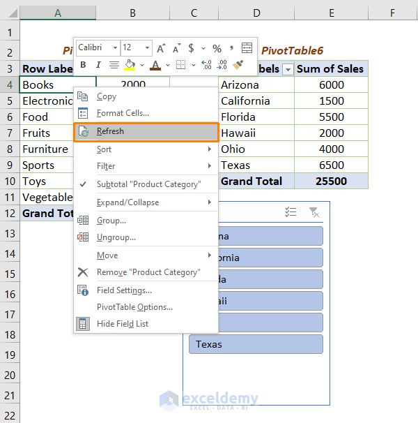
The Pivot Tables are updated.

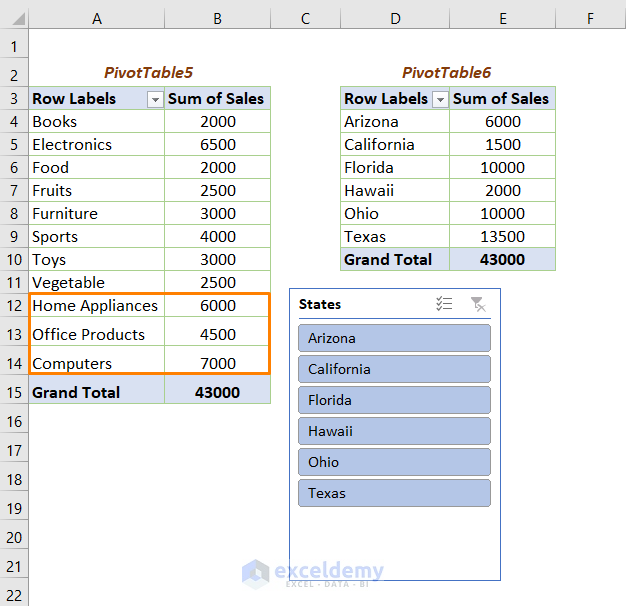
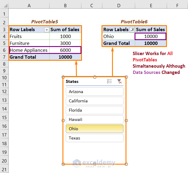
The Slicer works for all Pivot Tables at the same time.

Download Practice Workbook

Related Articles

• How to Change Slicer Color in Excel
• How to Resize a Slicer in Excel
• How to Insert Slicer without Pivot Table in Excel
• Connect Slicer to Multiple Pivot Tables from Different Data Source
• Excel Slicer for Multiple Pivot Tables (Connection and Usage)