Create Retirement Budget Worksheet in Excel (with Easy Steps)

Microsoft Excel is a powerful software. We can perform numerous operations on our datasets using Excel tools and features. There are many default Excel Functions that we can use to create formulas. Many educational institutions and business companies use Excel files to store valuable data. Even individuals sometimes need to have different Excel worksheets for their benefit. Each of those worksheets will serve a distinct purpose. Such a kind is the Retirement Budget Worksheet where we can estimate the post-retirement financial aspects. This article will show you the step-by-step procedures to create a Retirement Budget Worksheet in Excel.

Step-by-Step Procedures for Creating Retirement Budget Worksheet in Excel

The Retirement Budget worksheet is where we estimate the post-retirement earnings and spending for a sound financial future. This is important for any individual to plan this well ahead of time. In this way, one can cautiously consume their present resources. After we retire, our income sources and incomes will be limited. On the other hand, our medical expenses may increase by a considerable amount. So, it’s crucial to plan early to manage all these aspects. In this regard, a retirement budget worksheet can keep that in check. Therefore, go through the steps carefully to create the desired worksheet.

STEP 1: Add Heading & Age Info

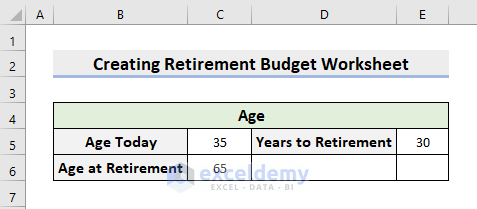
First, we’ll type the desired heading that’ll give users a clear understanding of the worksheet.
In our example, the heading is Creating Retirement Budget Worksheet.
Then, we’ll input the Age information.
This includes today’s age, age at retirement, and years left to retire from today.
See the below picture for a better understanding.

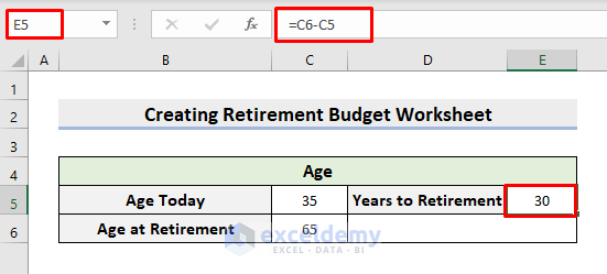
To calculate Years to Retirement, select cell E5.
Type the formula:

=C6-C5

Subsequently, press Enter.

STEP 2: Input Income

Now, we’ll input the income information.
Here, include all of your income sources and incomes by week, month, or year.
In our example, the Company Pension and the Social Security Income are two monthly income sources.

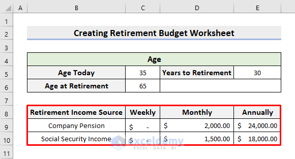
To determine the annual income from the monthly amount, we just need to multiply the figure by 12.
Look at the following dataset to make yourself clear.

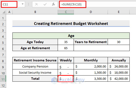
Next, we’ll compute the total income.
For this purpose, use the AutoSum feature in cell C11 which sums the cell range.
Accordingly, apply AutoFill to the right side to get the subsequent results.

STEP 3: Insert Payments

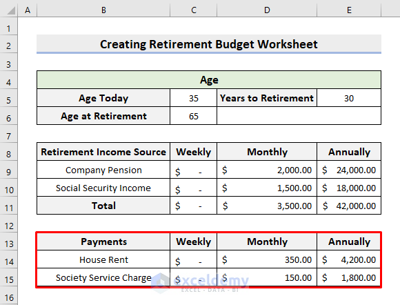
After the income section, we’ll add the Payments.
Here, the payments are the ones that are usually fixed amounts we have to pay within a definite time frame.
House Rent and Society Service Charges are the payments in our example and they are monthly payments.

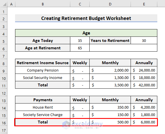
After that, we’ll determine the Total as we did in the income section.

STEP 4: Include Expenses

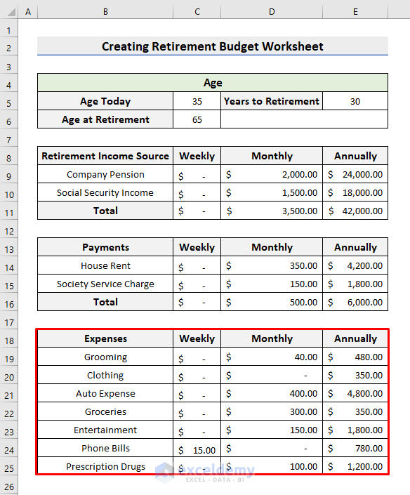
Similarly, we have to add the Expenses.
In this step, include all of your expense titles and amounts categorized as weekly, monthly, and annually.
Notice that some of the expenses can happen annually, like the clothing expenses in our dataset.

Again, to get the annual calculation from the weekly amount, such as for Phone Bills, select cell E24.
Then, input the formula:

=C24*52

Afterward, press Enter.
We multiply C24 by 52 because there are approximately 52 weeks in a year.

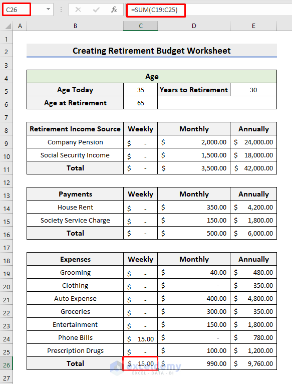
Subsequently, we’ll determine the Total Expenses by using the AutoSum feature.
Next, apply AutoFill.

STEP 5: Generate Summary

Lastly, we’ll generate the Summary section.
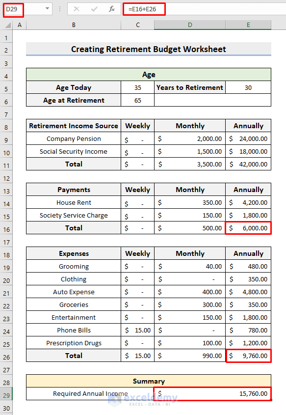
We’ll calculate the Required Annual Income first.
In this regard, click cell D29.
Then, type the formula:

=E16+E26

Hit Enter.
Here, this output is the sum of the expenses and the payments.

Next, we’ll determine the annual income that we receive.
So, in cell D30, input the formula:

=E11

Click Enter.
E11 is our sum of the incomes.

At last, we’ll compute the Annual Net Balance.
Accordingly, select cell D31.
Insert the formula:

=D30-D29

Press Enter.
Thus, you’ll get the net balance.

Final Output

Hence, our retirement budget worksheet is ready to be demonstrated. You can modify the template as per your own requirements. See the following worksheet which is our outcome.

Download Practice Template

Download the following template to practice by yourself.

Retirement Budget Worksheet.xlsx

Conclusion

Henceforth, you will be able to create a Retirement Budget Worksheet in Excel following the above-described steps. Keep using them and let us know if you have more ways to do the task. Don’t forget to drop comments, suggestions, or queries if you have any in the comment section below.