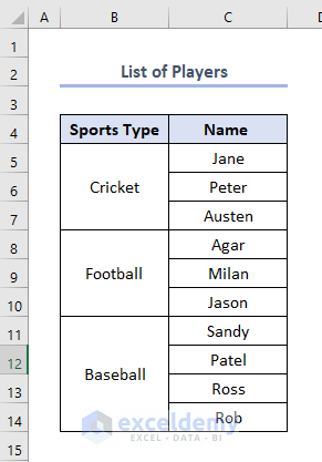
We have made a dataset as a List of Players.
Method 1 – Using the RAND Function to Randomly Select Names in Excel
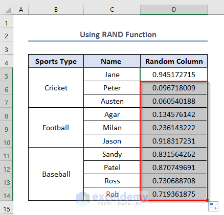
- Use the following formula in the D5 cell.
=RAND()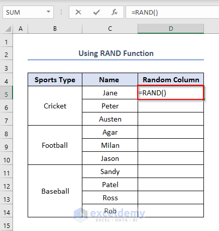
- Press Enter and use the Fill Handle by dragging the cursor while holding the bottom-right corner of the D5.
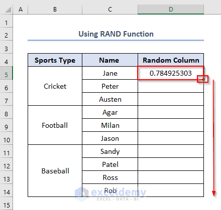
- We’ll get the outputs in the Random Column.
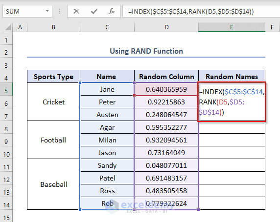
- Use the following formula using the INDEX and RANK functions in the E5 cell.
=INDEX($C$5:$C$14,RANK(D5,$D5:$D$14))Formula Explanation
- RANK(D5,$D5:$D$14)) → returns the rank of D5 e.0.640365959 among the values of cells D5:D14.
- $C$5:$C$14,RANK(D5,$D5:$D$14)) → returns the names in cells C5:C14 and then gives the rank of the name in D5 cell i.e. gives the rank of Jane.
- INDEX($C$5:$C$14,RANK(D5,$D5:$D$14)) → returns the intercept name which happens from the interception of the output value of $C$5:$C$14,RANK(D5,$D5:$D$14)) and the rows from C5:C14.
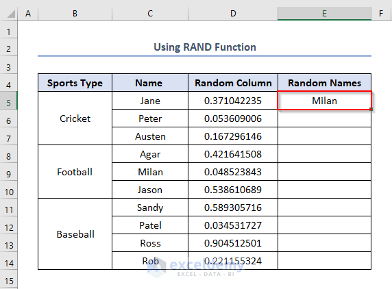
- Press Enter and use the Fill Handle to get other names randomly.
Method 2 – Utilizing INDEX, RANDBETWEEN, and COUNTA Functions to Randomly Select Names in Excel
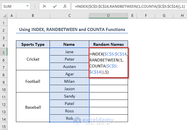
- Use the following formula in the D5 cell.
=INDEX($C$5:$C$14,RANDBETWEEN(1,COUNTA($C$5:$C$14)),1)Formula Explanation
- COUNTA($C$5:$C$14) → returns the number of counts from cell C5 to C14.
- Output → 10
- RANDBETWEEN(1,COUNTA($C$5:$C$14)) → returns any random value between 1 and
- INDEX($C$5:$C$14,RANDBETWEEN(1,COUNTA($C$5:$C$14)),1) → returns the intercept name which happens from the interception of the output value of RANDBETWEEN(1,COUNTA($C$5:$C$14)) and the rows from C5:C14.
- Hit Enter.
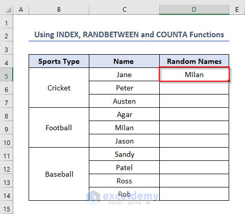
- Use the Fill Handle to get multiple outputs of random selected names.

Method 3 – Using INDEX, RANDBETWEEN, and ROWS Functions
- Use this formula in the D5 cell.
=INDEX($C$5:$C$14,RANDBETWEEN(1,ROWS($C$5:$C$14)))Formula Explanation
- ROWS($C$5:$C$14)→ Returns number of rows between cells C5 to C14.
- RANDBETWEEN(1,ROWS($C$5:$C$14))→ Returns a random number between 1 and number of rows.
- INDEX($C$5:$C$14,RANDBETWEEN(1,ROWS($C$5:$C$14)))→ The number returned by RANDBETWEEN is fed to the row_num argument of the INDEX function, so it picks the value from that row. In the column_num argument, we supply 1 because we want to extract a value from the first column.
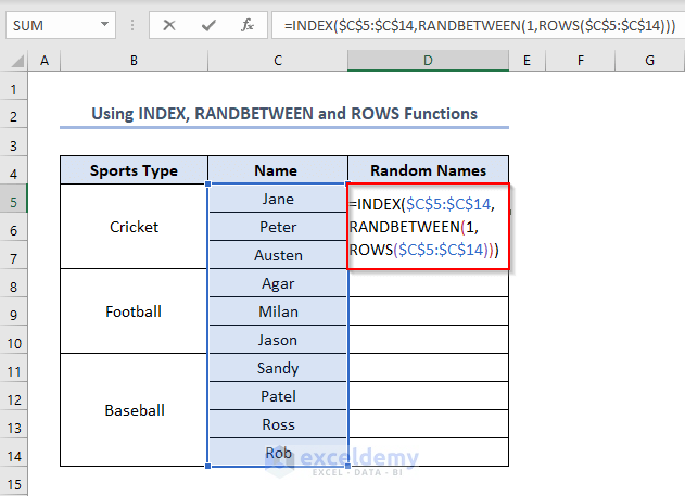
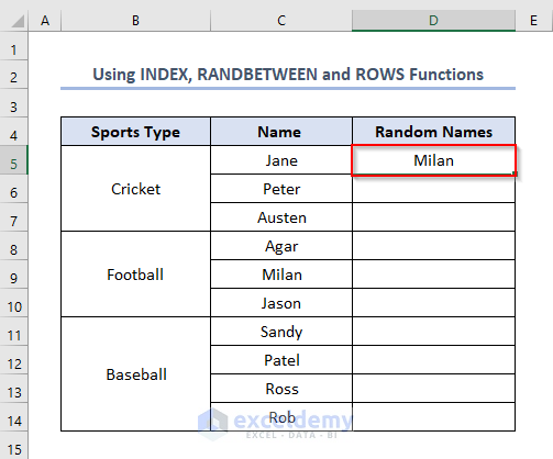
- Press Enter to get the random name as output.
Method 4 – Applying CHOOSE and RANDBETWEEN Functions to Randomly Select Names in Excel
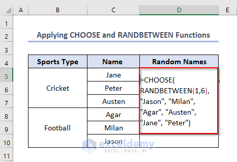
- Insert this formula in the D5 cell.
=CHOOSE(RANDBETWEEN(1,6), "Jason", "Milan", "Agar", "Austen", "Jane", "Peter")The parameter bottom of the RANDBETWEEN function is 1 and the top is 6. The result of this function is a random number between 1 and 6 which is the index_num parameter of the CHOOSE function. The values of the function are “Jason”, “Miller”, “Agar”, “Austen”, “Jane”, “Peter”.
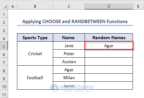
- Press Enter to find the output as a random name.
Method 5 – Using INDEX, RANK.EQ, and COUNTIF Functions
- Fill up the Random Column by using the RAND function.
- Insert the following formula in the E5 cell.
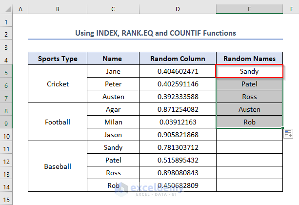
=INDEX($C$5:$C$14,RANK.EQ(D5,$D$5:$D$14)+COUNTIF($D$5:D5,D5)-1,1)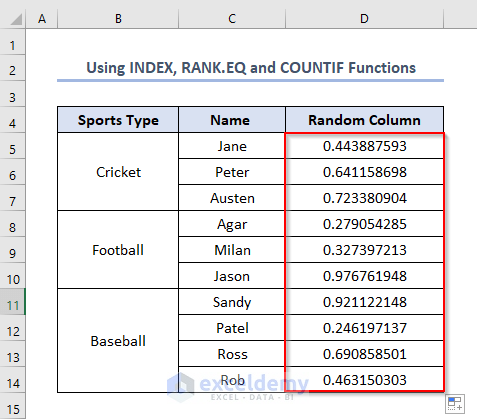
- Press Enter and use the Fill Handle to get all the outputs as random names.
Things to Remember
- If we use the combination of INDEX, RANDBETWEEN and COUNTA functions, we can get random names with duplicates i.e. one name can repeat several times.
- Using the RAND function gives the random names without duplication.
Download the Practice Workbook
<< Go Back to Random Selection in Excel | Randomize in Excel | Learn Excel
Get FREE Advanced Excel Exercises with Solutions!
