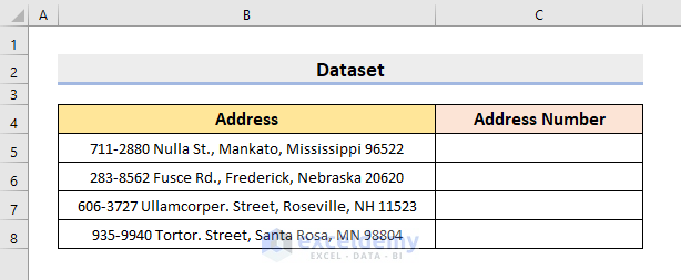
Suppose we have the following dataset. Let’s separate the Street Numbers in the Address column into column D.
Method 1 – Combining IF, ISERROR, VALUE, LEFT & FIND Functions
The IF function tests a condition, returns a value if the condition is satisfied, and another if it isn’t. The ISERROR function verifies whether a value is an error or not. The VALUE function converts a text string to a number. The LEFT function returns a specified number of characters from the start of a text string. The FIND function looks for a particular character in a text string and returns the position of that character.
Steps:
- Select cell C5.
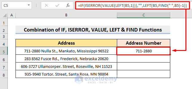
- Enter the following formula:
=IF(ISERROR(VALUE(LEFT(B5,1))),"",LEFT(B5,FIND(" ",B5)-1))- Press Enter to return the Address Number.
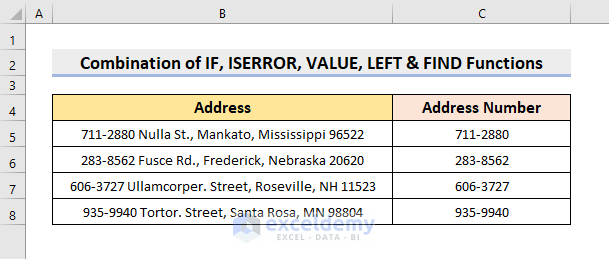
- Use the AutoFill tool to complete the rest of the column.
How Does the Formula Work?
- FIND(” “,B5)-1: Finds the position of the first space in B5 (returns 8 in this case) and subtracts 1 to determine the position before the space.
- LEFT(B5,FIND(” “,B5)-1): Extracts characters from the start of B5 up to the 7th position, resulting in “711-2880”.
- VALUE(LEFT(B5,1)): It evaluates the first character of B5. If numeric, it outputs the value (e.g., 7).
- ISERROR(VALUE(LEFT(B5,1))): Checks for errors in the VALUE function. Since “7” is numeric, this returns FALSE.
- IF(ISERROR(VALUE(LEFT(B5,1))),””,LEFT(B5,FIND(” “,B5)-1)): Uses the condition from ISERROR. If TRUE, it outputs an empty string. If FALSE, it returns the address number (“711-2880”).
Read More: How to Separate Address in Excel with Comma
Method 2 – Combining IF, ISNUMBER, VALUE, LEFT & FIND Functions
This method is almost the same as the previous one, except we’ll insert the ISNUMBER function instead of ISERROR. This function tests whether the argument is a number or not and returns True or False.
Steps:
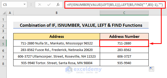
- In cell C5 enter this formula:
=IF(ISNUMBER(VALUE(LEFT(B5,1))),LEFT(B5,FIND(" ",B5)-1),"")- Press Enter to return the value.
- Use AutoFill to fill the rest.
The desired output is returned.
How Does the Formula Work?
- FIND(” “,B5)-1
This formula looks for space in B5 and returns 8.
- LEFT(B5,FIND(” “,B5)-1)
Generates 711-2880.
- VALUE(LEFT(B5,1))
The output is 7.
- ISNUMBER (VALUE(LEFT(B5,1)))
The output is True.
- IF(ISNUMBER(VALUE(LEFT(B5,1))),LEFT(B5,FIND(” “,B5)-1),””)
The IF function returns the outcome of LEFT(B5,FIND(” “,B5)-1) i.e 711-2880 as the condition is True.
Read More: How to Separate City and State in Excel
Method 3 – Using LEFT & FIND Functions
The formula in this method is very simple compared to the earlier ones.
Steps:
- In cell C5, enter the formula:
=LEFT(B5,FIND(" ",B5,1))- Press Enter.
- Use AutoFill to return the desired output.
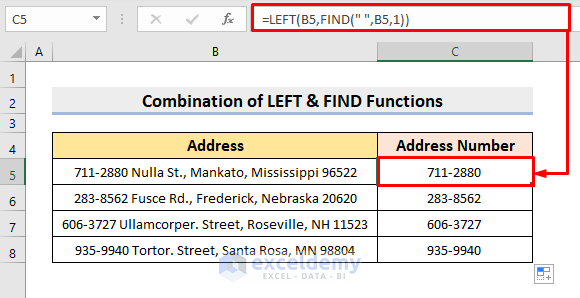
How Does the Formula Work?
- FIND(” “,B5)-1
Looks for space in B5 and returns 8.
- LEFT(B5,FIND(” “,B5)-1)
Generates 711-2880.
Read More: How to Separate City State and Zip from Address Using Excel Formula
Method 4 – Using Text to Columns Feature
Steps:
- Select the range B5:B8.
- Select Data ➤ Data Tools ➤ Text to Columns.
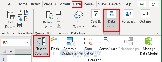
A dialog box will pop out.
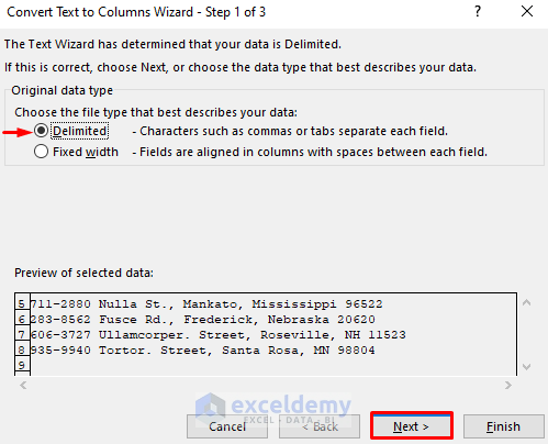
- Choose Delimited and click Next.
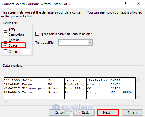
- Check the box for Space.
- Press Next.
- Select the desired destination and press Finish.
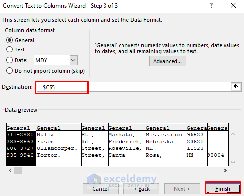
The Address Numbers will be extracted as below.

Read More: How to Separate Address in Excel
Method 5 – Using Excel VBA Code
Steps:
- Go to the Developer tab and select Visual Basic.

- In the pop-out VBA window, select Insert ➤ Module.
The Module dialog box will appear.
- Copy the below code and paste it into the box:
Sub SplitAddNum()
    Dim st As String
    Dim p As Integer
    Dim i As Integer
    For Each cell In Selection
        st = cell.Value
        p = InStr(st, " ")
        If p > 0 Then
            i = Val(Left(st, p))
            If i > 0 Then
                cell.Offset(0, 1).Value = i
                st = Trim(Mid(st, p, Len(st)))
            End If
        End If
        cell.Offset(0, 2).Value = st
    Next
End Sub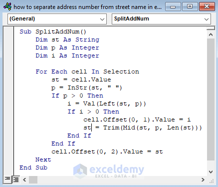
- Save the file and close the VBA window.
- Choose the range B5:B8.
- Click Developer ➤ Macros.
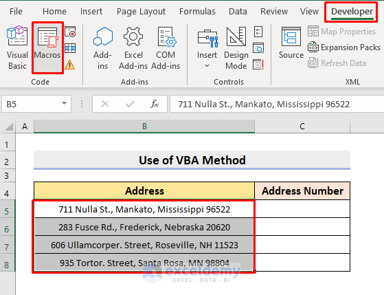
The Macro dialog box will appear.
- Select SplitAddNum and press Run.
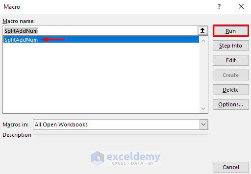
The macro will return the address number and the rest of the address in separate columns.
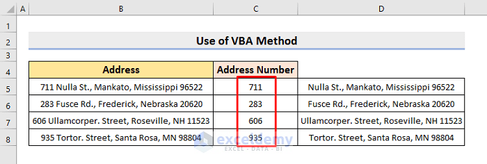
Read More: How to Split Inconsistent Address in Excel
Method 6 – Using Flash Fill Feature
Steps:
- Input the first row like in the following picture.

- Select cell C6 and go to Data ➤ Data Tools ➤ Flash Fill.
- Alternatively, press the Ctrl and E keys together.
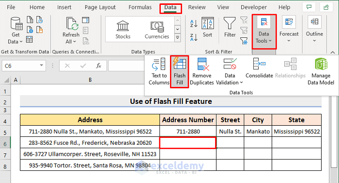
Our expected outcome is returned.

- Return the other fields by repeating the above steps.

Download Practice Workbook
Related Articles
- How to Separate Address in Excel Using Formula
- How to Separate City and State without Commas in Excel
<< Go Back to Address Format | Text Formatting | Learn Excel
Get FREE Advanced Excel Exercises with Solutions!


Thanks for the reference.
I noticed some unclear explanations:
How Does the Formula Work?
FIND(” “,B5)-1
This formula looks for space in B5 and returns 8.
Comment: the -1 subtracts 1 to find the place *before* the space.
LEFT(B5,FIND(” “,B5)-1)
Generates 711-2880.
Comment: “Generates 711-2880” doesn’t explain that the function cuts the characters * places from the left. In this example, the function uses the “8” to cut the 1st 8 characters from the left.
VALUE(LEFT(B5,1))
The output is 7.
Comment: Are you testing to see if the leading character in the character string is a number?
ISERROR(VALUE(LEFT(B5,1)))
The output is False.
Comment: ISERROR is looking for an error within the parentheses. In this case, the parenthetical contains an output of “7”. Therefore, the parenthetical does not produce “Error”and the “ISERROR” function returns “False”.
IF(ISERROR(VALUE(LEFT(B5,1))),””,LEFT(B5,FIND(” “,B5)-1))
Lastly, the IF function returns the outcome of LEFT(B5,FIND(” “,B5)-1) i.e 711-2880 as the condition is False.
Comment: This IF function uses the first parameter as the test. The ISERROR outcome is the function creating a F/T condition. If F, then follow the second parameter; and if T follow the third parameter. Since the condition produces a “F”, the first parameter’s results are the output. Result is “711-2880”.
Hello Chris,
Thank you for your detailed feedback! We’ve updated the article to provide clearer explanations for how the formula works, addressing your observations. Here’s a summary:
1. FIND and LEFT are used to locate and extract the address number.
2. VALUE checks if the first character is numeric.
3. ISERROR and IF determine if an address number exists and return it if valid.
We appreciate your input and invite you to revisit the updated explanation. Thank you for helping us improve!
Regards
ExcelDemy