How to Separate Date from Text in Excel (4 Methods)

Method 1 – Combining MID, SEARCH & DATEVALUE Functions to Separate Date from Text in Excel

Let’s consider the following dataset with dates inside other text in cells. Let’s extract the dates.

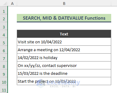
Steps:

• Copy the below formula in Cell C5 and hit Enter:

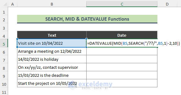
• We will get the below result. Here we received a numeric value—because Excel stores dates as a serial number—since the cell is in the Number format.

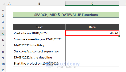
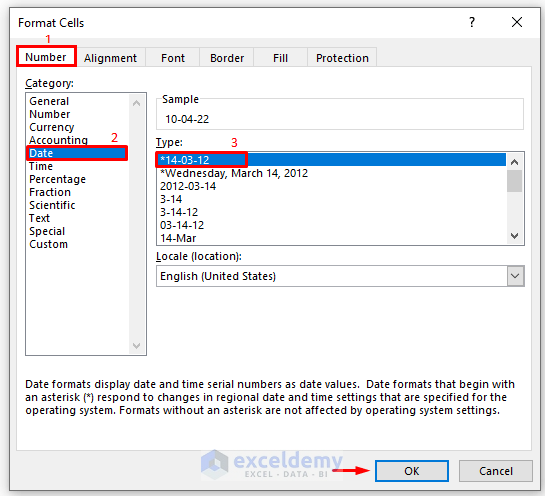
• Let’s convert the value into Date format. Select Cell C5 and press Ctrl + 1 to bring the Format Cells dialog.
• When the Format Cells dialog appears, go to the Number tab, select Category: Date and choose the date Type.
• Press OK.

• The previous numeric value is changed to a date.
• Use the Fill Handle (+) to replicate the cell formatting and formula to the other cells in the column.

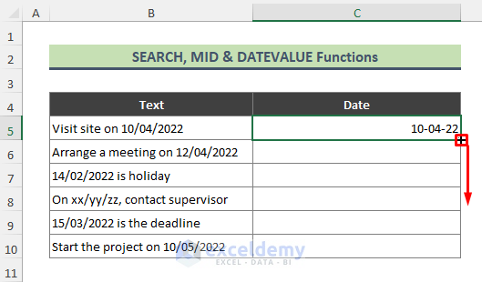
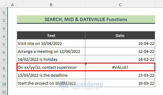
• There is a problem with the text string of Cell B8. As the date included in the string is not a valid date, Excel returns the #VALUE! error.

• Let’s modify the above formula with the IFERROR function. The final formula for the cells is:

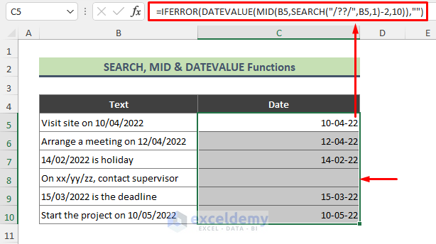
We can see that the IFERROR function returns a blank (“ “) when the result is an error.

How Does the Formula Work?

Method 2 – Joining Excel INDIRECT, LEN, MIN, FIND & ROW Functions to Separate Date from Text

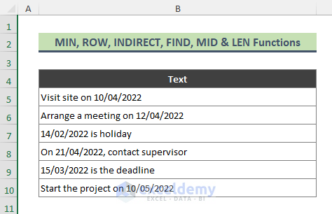
Suppose we have the below dataset containing several text strings that contain dates too.

Steps:

• Copy the below formula in Cell C5 and press Enter:

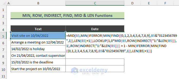
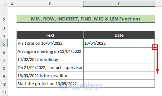
• We can see the date portion of the text of Cell B5 is separated as shown in the below screenshot.
• Use the Fill Handle (+) to copy the formula to the rest of the cells.

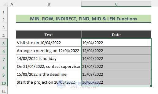
• We will get the below output. All the dates from each text string are separated.

How Does the Formula Work?

Method 3 – Applying Excel Text to Columns Tool to Separate Date from Text

Let’s say we have the below dataset containing several text strings along with date values.

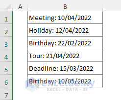
Steps:

• Select the column with the text strings (here, column B).

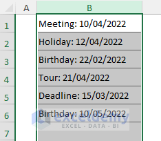
• Go to Data and select Text to Columns.

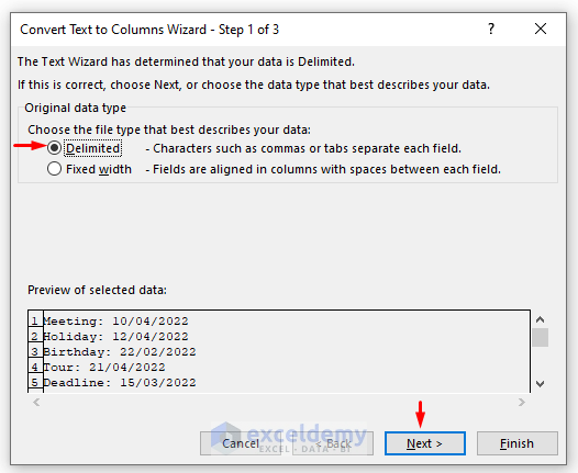
• The Text to Columns window appears. Choose the Delimited option and press Next.

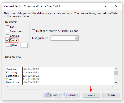
• From the Delimiters section, put a checkmark on Space and click Next.

• From the Column Data Format section, click on the Do not import column (skip), choose the destination location, and press Finish.

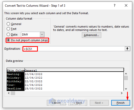
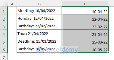
• Here is the output we receive. All the dates are extracted from the corresponding text strings.

Method 4 – Using VBA Macro to Separate Date from Text

Steps:

• Go to Developer and select Visual Basic. You can use Alt + F11, too, to bring the VBA window.

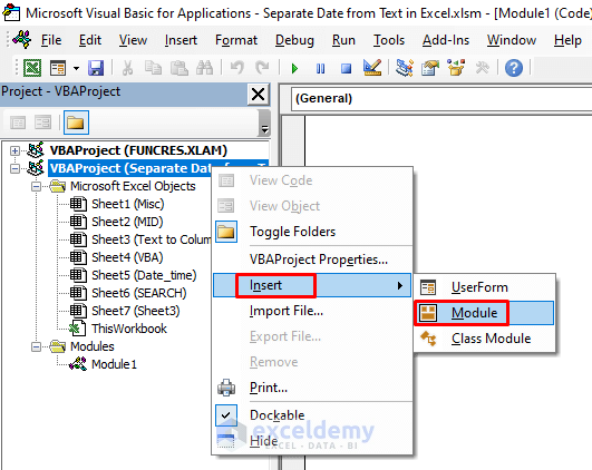
• When the VBA window shows up, right-click on VBAProject and select Insert, then choose Module.

• Copy the below code in the newly created Module and save it.

Function DateSeparate(st As String)
On Error GoTo eH
Dim j As Integer, d As Date, ar() As String, tmp As String
d = 0
ar = Split(st)
For j = LBound(ar) To UBound(ar)
tmp = ar(j)
If IsDate(tmp) And Len(tmp) > 5 Then
d = DateValue(tmp)
Exit For
End If
Next j
cont:
DateSeparate = d
Exit Function
eH:
d = 0
Resume cont
End Function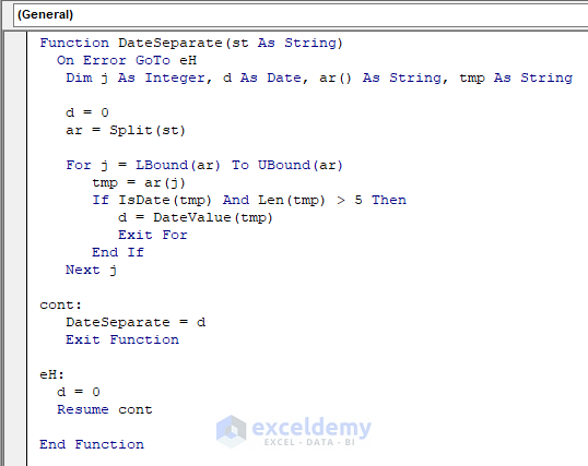

• Since this is a function, go back to the worksheet.
• Copy the below formula in Cell C5, and press Enter:

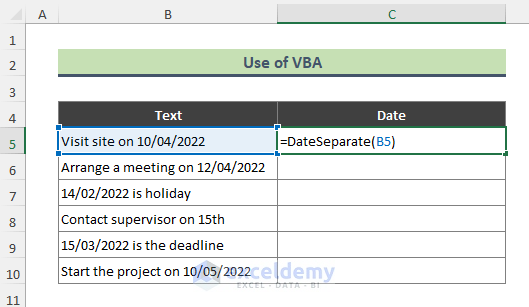
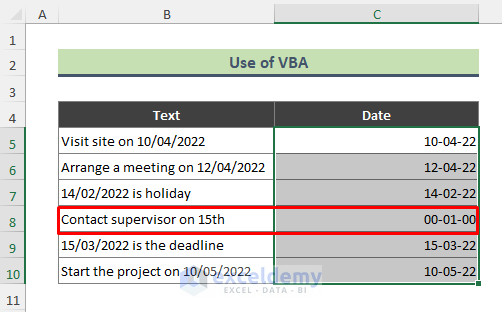
• We will get the below output (after converting to Date Number format). However, for the text of Cell C8, we do not get any valid date as the text does not have a regular date format.

• Wrap the UDF with the IF function to solve the issue. The new formula is:

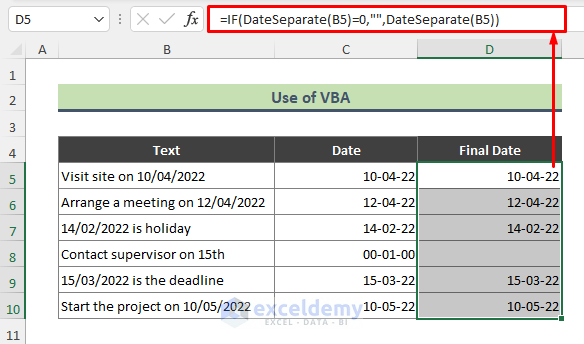
Here, the IF function returns blank (“ “) when the result of UDF is not a valid date.

How to Separate Date and Time in Excel

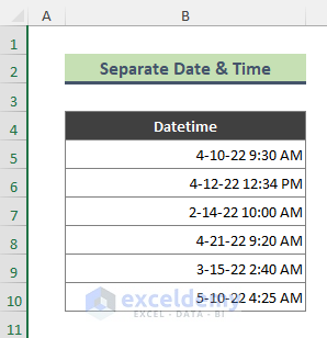
You can split the date and time from date-time using the INT function in Excel. Consider the following column with full times.

Steps:

• Convert the date-time data into General Number format.
• Use the below formula to get the date part of the date-time:

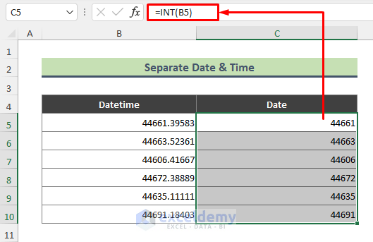
• The above result is in General Number format. Convert it to Date format.

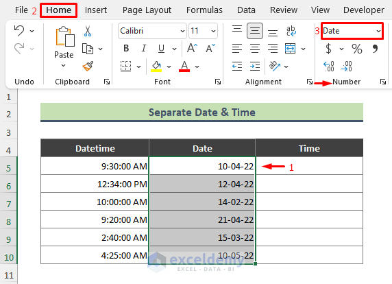
• Next, to find the time part of the date-time use the following formula:

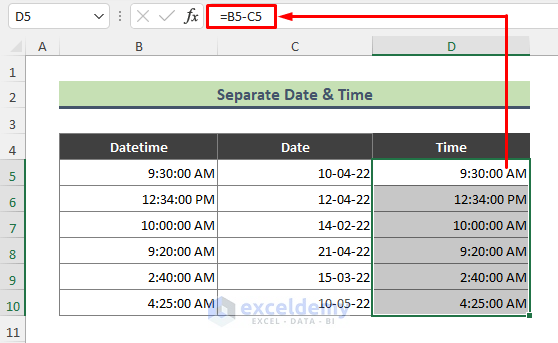
Download Practice Workbook

You can download the practice workbook that we have used to prepare this article.

<< Go Back to Date and Time | Split | Learn Excel