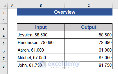
This article will show how to separate decimal numbers from text in Excel, like in the following image.
Method 1 – Using Text to Column Wizard
The Text to Column feature is used to separate a specific section from data in Excel.
Steps:
- Add a column named Decimal Number to show the decimal numbers only.
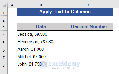
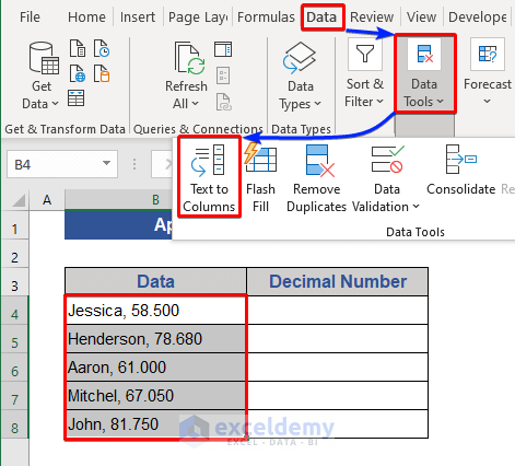
- Select all the cells of the Data column.
- Go to the Data tab.
- Choose the Text to Columns button from the Data Tools group.
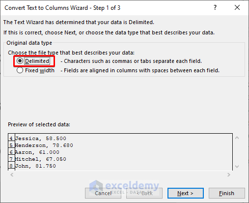
- Choose the Delimited option and then press Next.
- Choose the Comma option.
- Press Next.
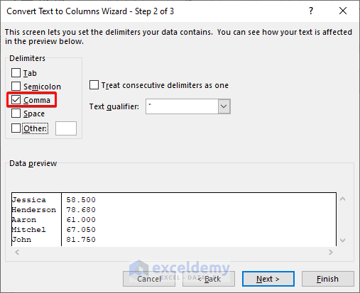
- Choose the General option.
- Choose the desired data from the Data preview section.
- Click the Finish button.
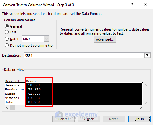
The decimal numbers are separated.
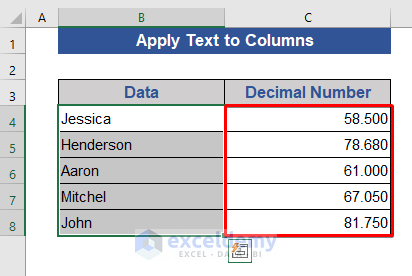
Method 2 – Using Flash Fill
The Flash Fill feature can sense patterns and automatically fill data according to a given pattern.
Note:
Flash Fill is only available in Excel 2013 and later versions.
Steps:
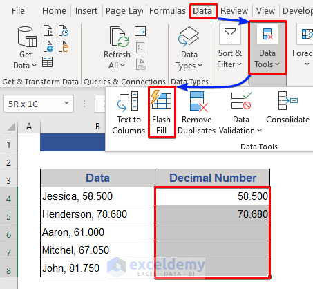
- Fill the first two cells of the Decimal Number column by manually entering the decimal numbers from the corresponding Data column.
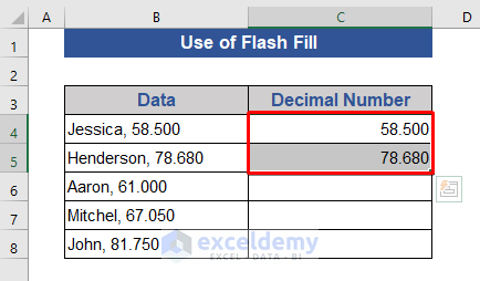
- Choose all the cells of the Decimal Number column.
- Go to the Data tab.
- Choose the Flash Fill option from the Data Tools group, or use the keyboard shortcut Ctrl+E.
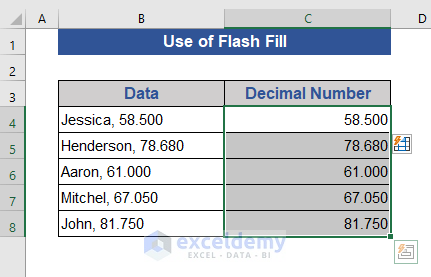
All the decimal numbers are separated.
Method 3 – Using a Formula Combining RIGHT, LEN, MIN, and FIND Functions
The FIND function returns the starting position of one text string within another text string, and is case-sensitive.

The MIN function returns the smallest number in a set of values and ignores logical values and text.

The LEN function returns the number of characters of a text string.

The RIGHT function returns the specified number of characters from the end of the text string.

Steps:
- In cell C4 enter the following formula:
=RIGHT(B4,LEN(B4)-MIN(FIND({0,1,2,3,4,5,6,7,8,9},B4&"0123456789"))+1)
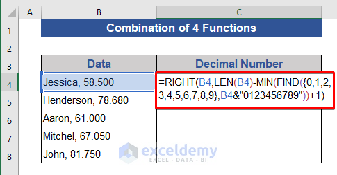
- Press Enter.
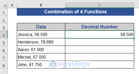
The decimal number in cell B4 is returned.
- Drag the Fill Handle icon down to copy the formula to the rest of the cells.
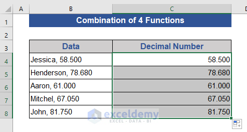
Formula Breakdown:
- FIND({0,1,2,3,4,5,6,7,8,9},B4&”0123456789″)
This will search for the 1st argument within the second argument.
Result: {14, 17, 18, 19, 20, 10, 22, 23, 11, 25}
- MIN(FIND({0,1,2,3,4,5,6,7,8,9},B4&”0123456789″))
This will return the minimum value from the given argument.
Result: 10
- LEN(B4)
This will return the length of cell B4.
Result: 15
- LEN(B5)-MIN(FIND({0,1,2,3,4,5,6,7,8,9},B5&”0123456789″))
A subtraction operation is performed here.
Result: 5
- RIGHT(B4,LEN(B4)-MIN(FIND({0,1,2,3,4,5,6,7,8,9},B4&”0123456789″))+1)
This will return the last 6 characters from cell B4.
Result: 58.500
Method 4 – Combining LEFT, LEN, SUM, and SUBSTITUTE Functions
The LEFT function returns the specified number of characters from the start of the text string.

The SUM function adds all the numbers from a range of cells.

The SUBSTITUTE function replaces existing text with new text in a text string.

In the previous method, we applied a formula to separate the decimal numbers from the right side. Now we will extract decimal numbers from the left side.
Steps:
- In cell C4 enter the following formula:
=LEFT(B4,SUM(LEN(B4)-LEN(SUBSTITUTE(B4,{"0","1","2","3","4","5","6","7","8","9"},"")))+1)
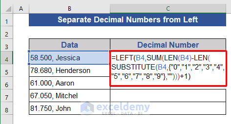
- Press Enter and drag the Fill Handle icon.
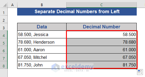
Decimal numbers are extracted from the left side.
Formula Breakdown:
- SUBSTITUTE(B4,{“0″,”1″,”2″,”3″,”4″,”5″,”6″,”7″,”8″,”9″},””)
This will replace the numerical values from cell B4.
Result: {58.5, Jessica; 58.500, Jessica; 58.500, Jessica; 58.500, Jessica; 58.500, Jessica; 8.00, Jessica; 58.500, Jessica; 58.500, Jessica; 5.500, Jessica; 58.500, Jessica}
- LEN(SUBSTITUTE(B4,{“0″,”1″,”2″,”3″,”4″,”5″,”6″,”7″,”8″,”9″},””))
This will find the length of the given reference.
Result: {13, 15, 15, 15, 15, 13, 15, 15, 14, 15}
- LEN(B4)
This will return the length of Cell B4.
Result: 15
- LEN(B4)-LEN(SUBSTITUTE(B4,{“0″,”1″,”2″,”3″,”4″,”5″,”6″,”7″,”8″,”9″},””))
A subtraction operation is performed here.
Result: {2, 0, 0, 0, 0, 2, 0, 0, 1, 0}
- SUM(LEN(B4)-LEN(SUBSTITUTE(B4,{“0″,”1″,”2″,”3″,”4″,”5″,”6″,”7″,”8″,”9″},””)))
A sum operation is performed using the result of subtraction.
Result: 5
- LEFT(B4,SUM(LEN(B4)-LEN(SUBSTITUTE(B4,{“0″,”1″,”2″,”3″,”4″,”5″,”6″,”7″,”8″,”9″},””)))+1)
This will return the first 6 characters from cell B4.
Result: 58.500
Method 5 – Combining ROW, MID, INDIRECT, and LOOKUP Functions
To extract decimal numbers from any location, use the following formula combining the ROW, MID, INDIRECT, and LOOKUP functions.
The ROW function returns the row number of a reference.

The MID function returns the character from the middle of a text string, given a starting position and length.

The INDIRECT function returns the reference specified by a text string.

The LOOKUP function looks up a value either from a one-row or one column range or from an array, provided for backward compatibility.

To illustrate this method, we will use the modified dataset below.
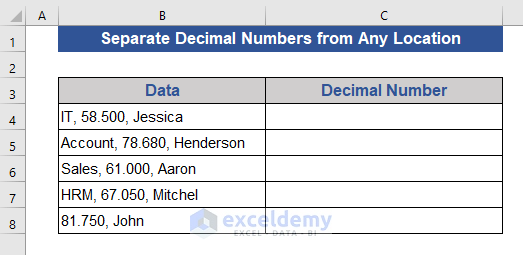
Steps:
- In cell C4 enter the formula below:
=LOOKUP(9.9E+307,--LEFT(MID(B4,MIN(FIND({1,2,3,4,5,6,7,8,9,0}, $B4&"1023456789")),999),ROW(INDIRECT("1:999"))))
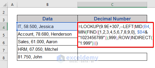
- Press Enter and drag the Fill Handle icon down.
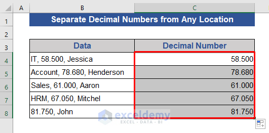
The decimal numbers from any location are returned.
Formula Breakdown:
- ROW(INDIRECT(“1:999”))
This provides numbers from 1 to 999.
- MIN(FIND({1,2,3,4,5,6,7,8,9,0}, $B4&”1023456789″))
This will return the minimum value from the results of the FIND function.
Result: 5
- LEFT(MID(B4,MIN(FIND({1,2,3,4,5,6,7,8,9,0},$B4&”1023456789″)),999),ROW(INDIRECT(“1:999”)))
This will return values from the left side.
- LOOKUP(9.9E+307,–LEFT(MID(B4,MIN(FIND({1,2,3,4,5,6,7,8,9,0}, $B4&”1023456789″)),999),ROW(INDIRECT(“1:999”))))
This will look up the decimal values from cell B4 and return those values.
Result: 58.500
Method 6 – Using VBA Code
Steps:
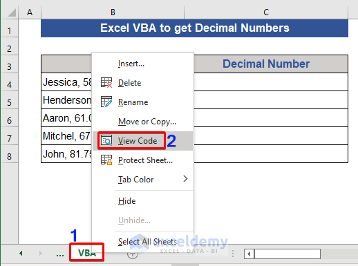
- Go to the Sheet name section at the bottom of each sheet and right-click the mouse.
- Choose the View Code option from the Context menu.
- Choose the Module option from the Insert tab of the VBA window.
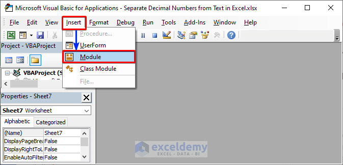
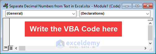
The VBA module appears. We will write the VBA code in this window.
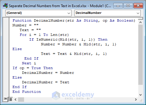
- Copy and paste the following VBA code into the module and Save the code:
Function DecimalNumber(str As String, op As Boolean)
Number = ""
   Text = ""
   For i = 1 To Len(str)
       If IsNumeric(Mid(str, i, 1)) Then
            Number = Number & Mid(str, i, 1)
Else
            Text = Text & Mid(str, i, 1)
     End If
    Next i
If op = True Then
    DecimalNumber = Number
Else
    DecimalNumber = Text
End If
End Function
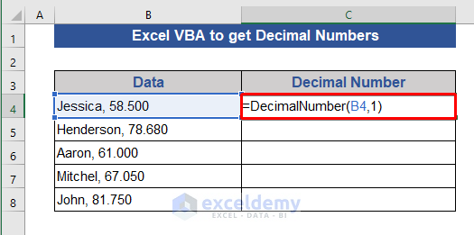
- Go to the dataset and enter the following formula in cell C4:
=DecimalNumber(B4,1)
- Press Enter and pull the Fill Handle icon down.
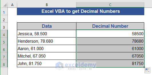
There is a difference here. In the result we get only the numbers without the decimal symbol.
Download Practice Workbook
<< Go Back to Separate Numbers Text | Split | Learn Excel
Get FREE Advanced Excel Exercises with Solutions!

