How to Solve Algebraic Equations with Multiple Variables (3 Ways)

Need to learn how to solve algebraic equations with multiple variables in Excel? If you are looking for such unique tricks, you’ve come to the right place. Here, we will take you through 3 easy and effective methods of solving algebraic equations with multiple variables.

Download Practice Workbook

You may download the following Excel workbook for better understanding and practice yourself.

3 Methods to Solve Algebraic Equations with Multiple Variables

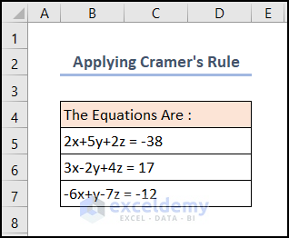
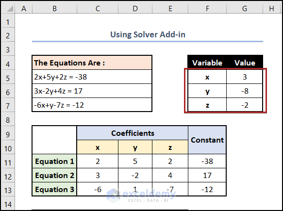
Let’s say we have the following three equations.
2x + 5y + 2z = -38
3x – 2y + 4z = 17
-6x + y – 7z = -12
Now, we’ll solve the equations by the following three methods. Thus, we’ll determine the value of the three variables x, y, and z.
Here, we have used Microsoft Excel 365 version, you may use any other version according to your convenience.

1. Applying Cramer’s Rule to Solve Algebraic Equations with Multiple Variables in Excel

Cramer’s rule is a particular formula in linear algebra. We often use it to solve systems of linear equations with as many equations as unknowns. It is effective whenever the equations have a distinct solution. Here, we’ll execute the same process just in Excel. So, follow these simple steps.

📌 Steps:

• At the very beginning, write down the equations in cells in the B5:B7 range.

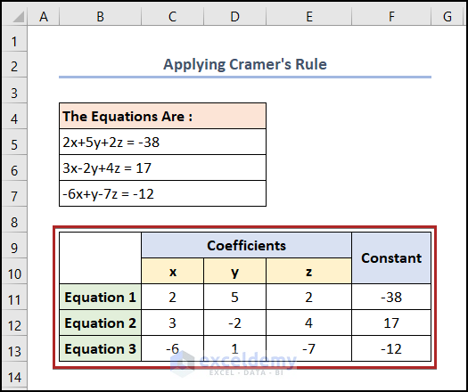
• Secondly, make a simple data range like in the image below.
• Here, in cells in the C11:E13 range, we insert the Coefficients of the variables x, y, and z.
• Also, in cells in the F11:F13 range, we input the Constants. Actually, they are the right-hand sides of the equations.

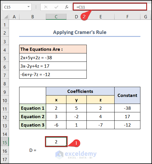
• At this moment, select cell C15 and put in the following formula.

• Then, press the ENTER key.

• In this instance, drag the Fill Handle tool up to cell E17 in two steps. Firstly, drag it vertically down. Then, move it horizontally to the right.
• Thus, you’ll get the coefficients in these cells.

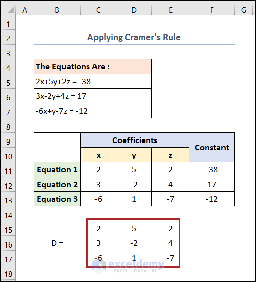
• Next, select cells in the C15:E17 range.
• Later, press CTRL+1.

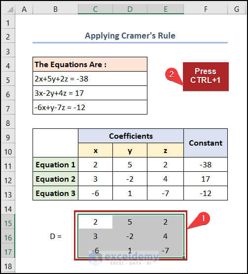
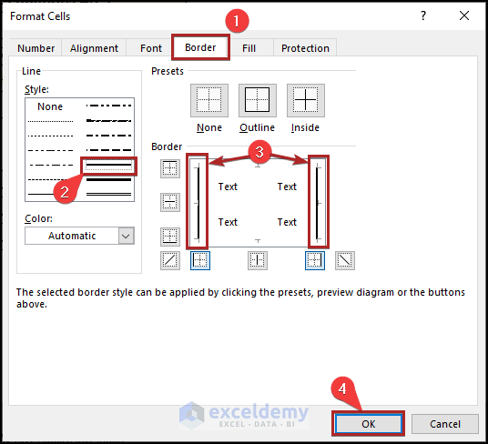
• Suddenly, it opens the Format Cells dialog box.
• After that, move to the Border tab.
• Then, select the Style as shown in the picture below.
• Later, give two outside borders like in the image.
• Lastly, click OK.

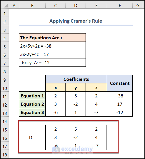
• Now, the data range looks like a determiner.

• Then, select cell C19 and write down the following formula.

• Then, press ENTER.
• Actually, here we’re putting the Constants in the first column.

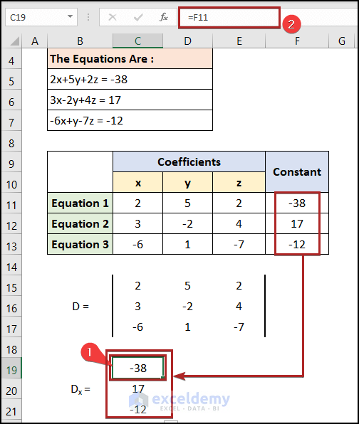
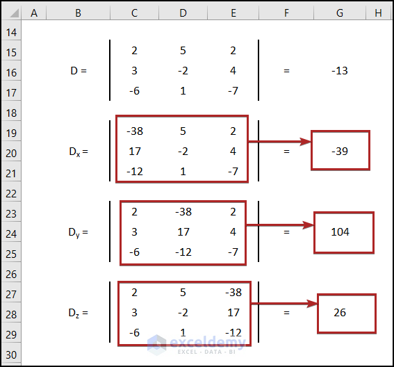
Note: In D_x, constants will sit in the first column. The coefficients of y and z will occupy the next two columns.

• At this time, put the coefficients of y and z in the next two columns.

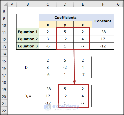
• In D_y, the constants will sit in the second column. The other two columns get occupied by the coefficients of x and z respectively.

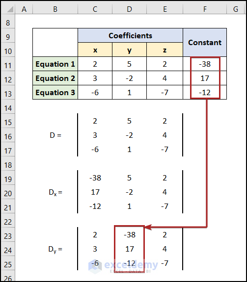
• Similarly, in D_z, the constants will sit in the third column. The other two columns get occupied by the coefficients of x and y respectively.

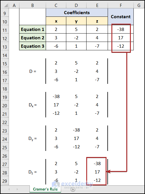
• Then, select cell D16 and get the following formula in the Formula Bar.

The MDETERM function determines the determinant of an array.

• Now, press ENTER.

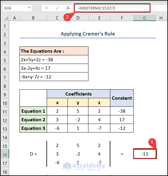
So, the determinant is -13.

• Similarly, calculate the determinant of x, y, and z also.

• Then, select cell G5 and paste the formula below.

• Hence, press ENTER.

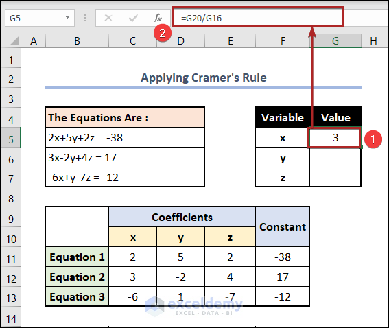
That’s how we get the value of variable x.

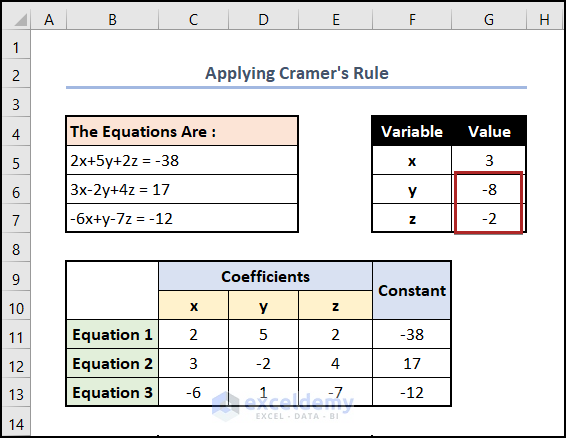
• Similarly, find the value of y and z by dividing their determinant (D_y; D_z) with the determinant D respectively.

Read More: How to Solve an Equation for X When Y is Given in Excel

2. Utilizing MINVERSE and MMULT Functions

In this method, we’ll use some Excel functions to solve the problem. Let’s see the process in detail.

📌 Steps:

• First of all, create a simple data range containing the Coefficients and Constants of the three equations like Method 1.

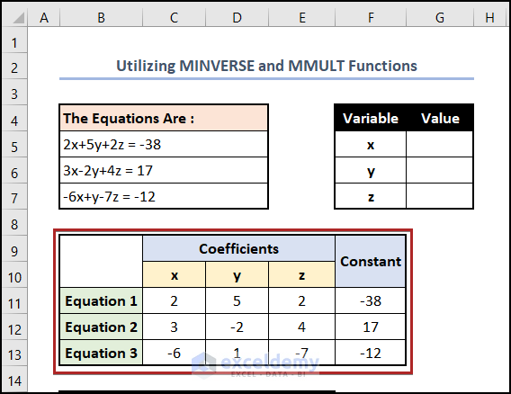
• Then, create matrix A and matrix B as in the image below.
• Here, matrix A contains the coefficients of the variables.
• On the other hand, matrix B includes the constants of the equations.

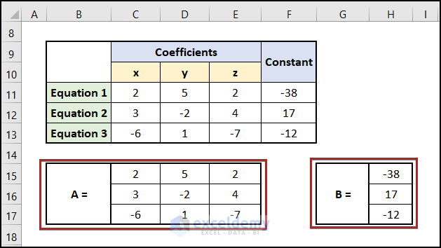
• Afterward, create a space for the inverse matrix of A.

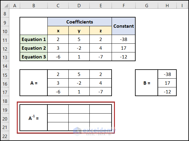
• Then, select cell C19 which is the first cell in this area.
• Later, write down the following formula.

The MINVERSE function returns the inverse matrix of a matrix. The main matrix should be stored in an array.

• Lastly, press ENTER.

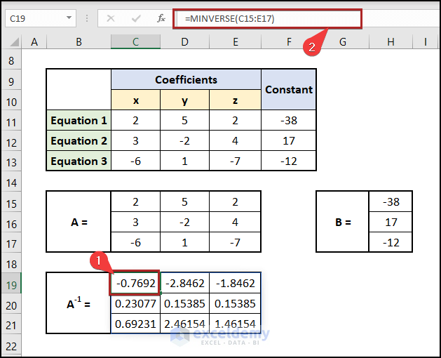
Note: If you are using any other version of Excel rather than Microsoft Excel 365, make sure to press CTRL+SHIFT+ENTER to get the result.

• Eventually, select cell G5 and paste the following formula.

Here, the MMULT function multiplies two matrices in array form. Then, it returns the product in also an array form.

• Correspondingly, hit the ENTER key.

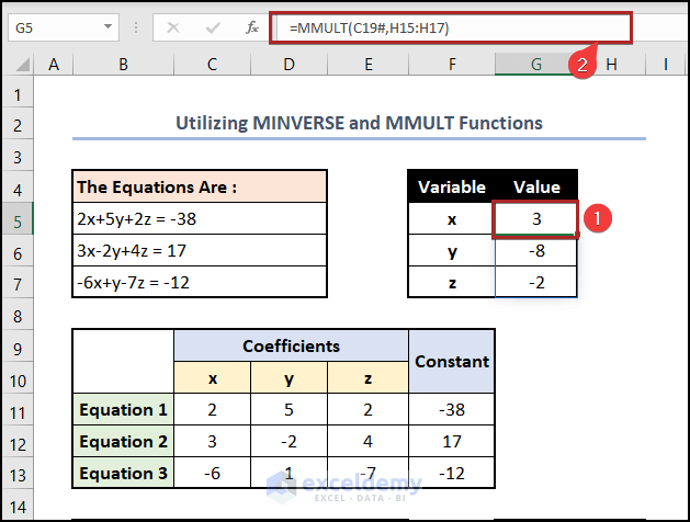
Thus, we get the values of the variables in cells in the G5:G7 range.

Read More: How to Solve For x in Excel (2 Simple Ways)

3. Using Solver Add-in to Solve Algebraic Equations with Multiple Variables in Excel

In this method, we’ll use an add-in of Excel. It’s the Solver add-in. So, without further delay, let’s dive in!

📌 Steps:

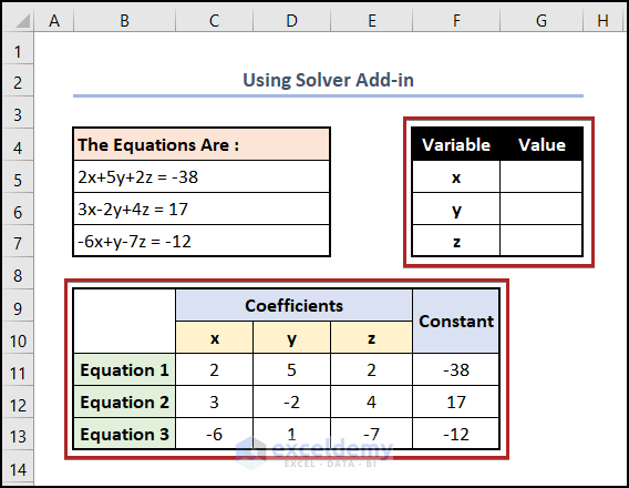
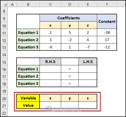
• Primarily, create a basic outline like in the image below. Also, we did it in Method 1.

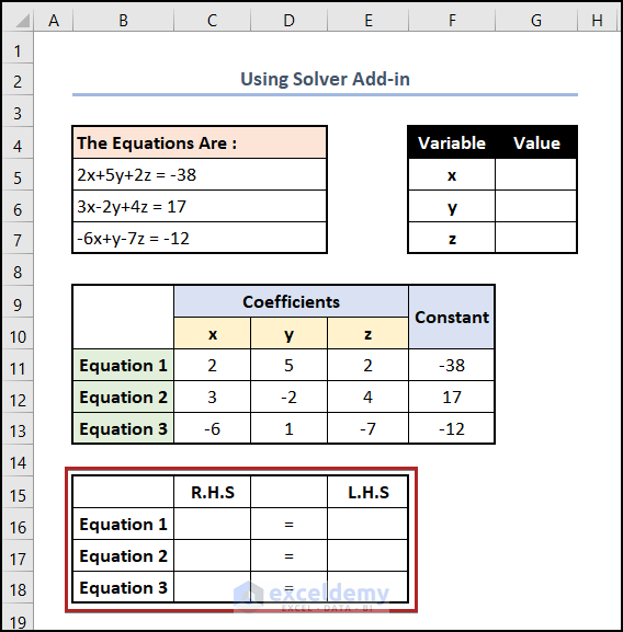
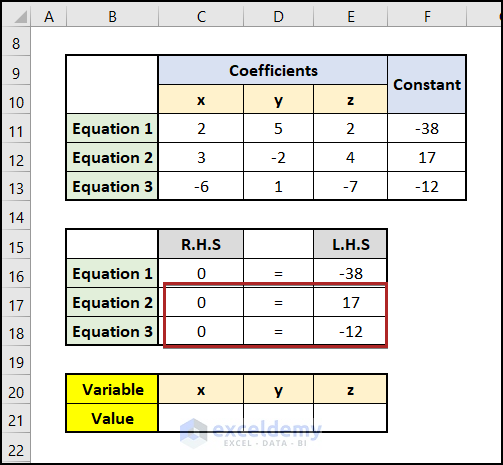
• Now, construct a data range like the below.
• It should contain the headings R.H.S, L.H.S horizontally and Equation 1, Equation 2, and Equation 3 vertically.

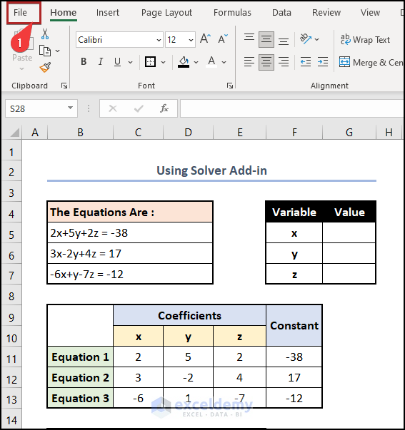
• Later, go to the File tab.

• Then, select Options from the menu.

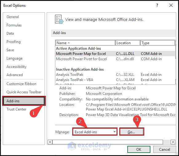
• Instantly, the Excel Options window opens up.
• Then, move to the Add-ins menu.
• After that, select Excel Add-ins from the Manage drop-down list.
• Later, click on Go.

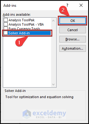
• Immediately, it opens the Add-ins dialog box.
• Now, check the box of Solver Add-in.
• Lastly, click OK.

• At this moment, create a data range like the picture below.

• Then, select cell C16 and insert the following formula.

Here, the SUMPRODUCT function returns the sum of the products of the corresponding values from all the arrays. It takes one or more arrays as an argument, multiplies the corresponding values of all the arrays, and then returns the sum of the products.

• As always, tap the ENTER key on your keyboard.

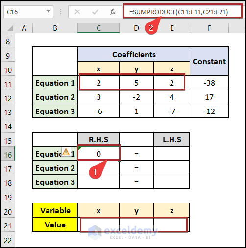
Note: For your convenience, we highlighted the cell ranges of the arguments in the picture above.

• After that, put the constant of Equation 1 in cell E16.

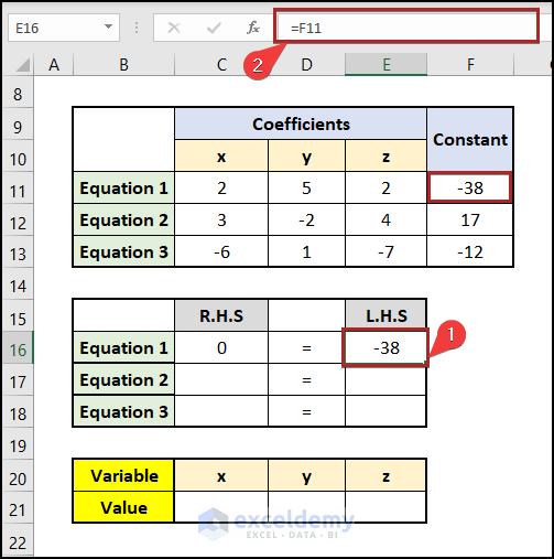
• Equivalently, fill up the fields of Equation 1 and Equation 2.

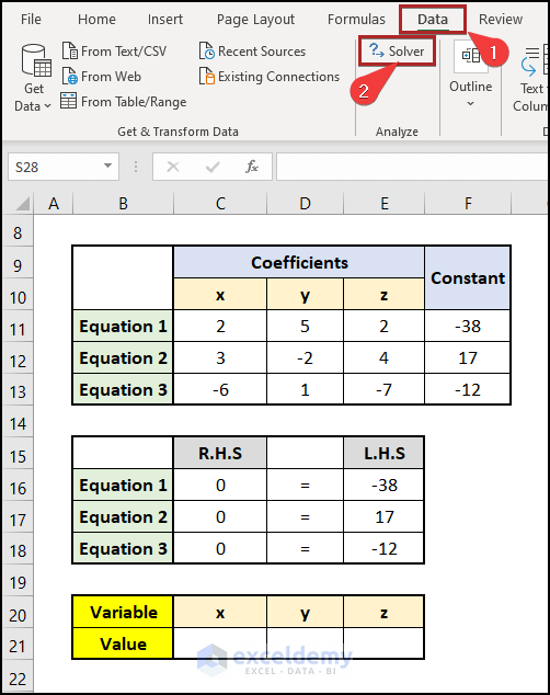
• Then, jump to the Data tab.
• Next, select Solver on the Analyze group.

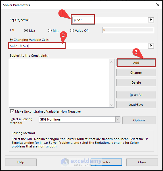
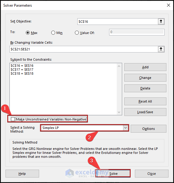
• Hence, the Solve Parameters wizard opens.
• Then, select cell C16 in the Set Objective box.
• After that, select cells in the C21:E21 range in the By Changing Variable Cells box.
• Lastly, click on the Add button.

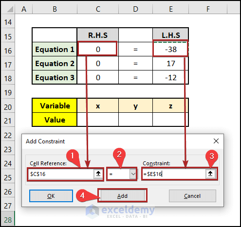
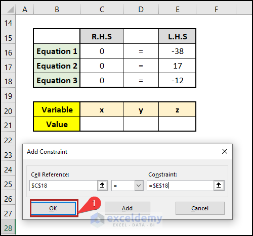
• Thus, it opens the Add Constraint input box.
• Later, give the reference of cell C16 into the Cell Reference box.
• Next, select the equal sign (=).
• After that, give the cell reference of cell E16 into the Constraint box.
• Lastly, click on Add.

• Correspondingly, repeat the above steps for Equation 2 and Equation 3.
• At last, click on the OK button.

• Again, it returns us to the Solver Parameters window.
• Then, untick the box of Make Unconstrained Variables Non-Negative.
• After that, choose Simplex LP from the Select a Solving Method drop-down list.
• Lastly, click on Solve.

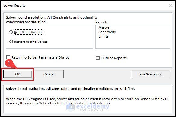
• Hence, the Solver Results wizard will open.
• Here, select the OK button.

• Thus, we can see the values of the variables in cells in the C21:E21 range.

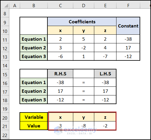
• Finally, move the answers to the top of the sheet to make them visible easily.
• So, transfer them to cells in the G5:G7 range.

That’s how we can solve these algebraic equations with multiple variables.

Read More: How to Solve 2 Equations with 2 Unknowns in Excel (2 Examples)

Practice Section

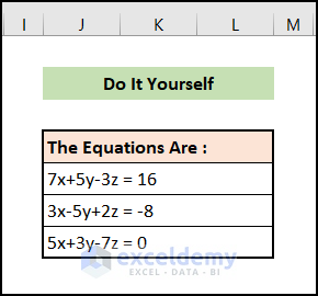
For doing practice by yourself we have provided a Practice section like below in each sheet on the right side. Please do it by yourself.

Conclusion

This article provides easy and brief solutions to solve algebraic equations with multiple variables in Excel. Don’t forget to download the Practice file. Thank you for reading this article, we hope this was helpful. Please let us know in the comment section if you have any queries or suggestions. Please visit our website Exceldemy to explore more.

Related Articles

• How to Solve Colebrook Equation in Excel (3 Simple Ways)
• Solve Quadratic Equation in Excel VBA (with Quick Steps)
• How to Solve Exponential Equation in Excel (4 Suitable Examples)
• Solve Cubic Equation in Excel (2 Ways)
• How to Solve Polynomial Equation in Excel (5 Simple Methods)
• Solve Differential Equation in Excel (With Easy Steps)