How to Subtract Two Columns in Excel (4 Easy Ways)

Q: Can I automate the subtraction process if new data is added to columns?

Using Excel Table (Ctrl+T), formulas will extend automatically when new data is added to the columns, facilitating the subtraction process.

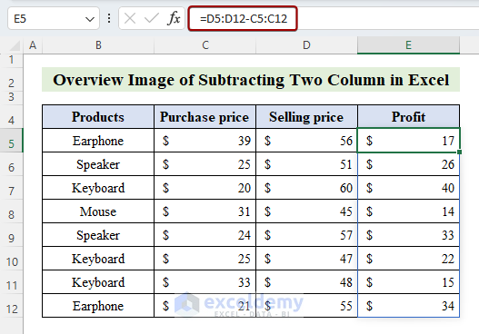
To subtract two columns in Excel:

Select a blank cell and insert the formula with the references for the columns such as: =A1-B1, then use the Fill Handle tool to copy the formula.
If you are using Microsoft 365, insert the array formula: =[Column 1] – [Column 2]. For example, [Column 1] = A1:A10 and [Column 2] = B1:B10

Let’s dig deeper into the subject and use a few different methods to subtract columns.

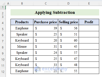
Consider a dataset where we have the Purchase price and Selling price for some products. By subtracting the two columns, we can obtain profit for each product.

Method 1 – Using the Subtraction Operator

Let’s use the provided dataset to calculate the profit on each item.

Select cell E6 and insert the formula: =D5-C5
Drag down the Fill Handle to copy the formula.

If you have Microsoft 365, you can subtract two columns in Excel by selecting a whole column and subtracting it from another. Therefore, you will get the whole outcome with an array format. Here’s how:

Select E6.
Insert the formula: =D5:D12-C5:C12
The formula returns an array format.

Note:

For any older versions other than Microsoft 365, press Ctrl + Shift + Enter keys for an array format.
The array formula returns a #SPILL! error if it can’t fit its contents.

Method 2 – Using the Absolute Cell Reference to Subtract

Select a cell D5 and insert the formula: =C5-$C$14
Apply the Fill Handle to copy the formula.
This subtracts the cell C14 from cells C5 to C13 and applies the result in column D.

Method 3 – Subtracting Two Columns with Dates

Select a cell D5 and apply the formula: =C5-B5
Use the Fill Handle tool to copy the formula in the adjacent cells.

For further calculation, the text format will not work. So, converting into a Number format is inevitable. Using the Excel VALUE function, you can subtract two columns and convert them into the number format:

Select a blank cell and insert the following formula: =VALUE(C5-B5)
Use the Fill Handle tool to copy the formula.
Thus, all the calculated values will be in number format.

Method 4 – Using the Paste Special Feature

Suppose we have a dataset of some products and their sales for two months. Let’s subtract a single cell value from all the columns.

Select the cell that you want to subtract from two columns and press Ctrl + C to copy.
Select the data from where you want to subtract.
Go to Home, choose the Paste drop-down, and select Paste Special.
The Paste Special dialog box appears.
Select the Subtract operation and click OK.
Therefore, we obtain the updated values by subtracting a fixed value from the two columns.

Method 5 – Using an Excel Pivot Table Tool to Subtract Two Columns

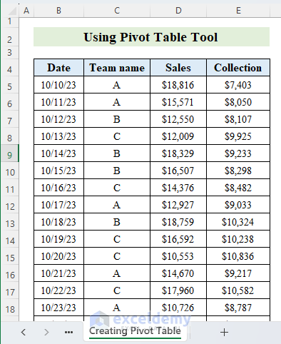
Suppose we have a dataset of some teams and their sales and collection reports. We will create a pivot table from the list and then subtract between the columns.

Step 1 – Create a Pivot Table

Select the whole dataset.
Go to the Insert tab and the PivotTable drop-down, then choose From Table/Range.
The PivotTable from table or range dialog box will appear.
Select the Existing Worksheet option and a location in the same worksheet.
Press OK.

Step 2 – Add the Pivot Table Fields

Check necessary components from the PivotTable Fields.

Step 3 – Create a New Calculated Field

Go to PivotTable Analyze, choose the Field, Items, & Sets drop-down and select Calculated Field.

A dialog box will appear named Insert Calculated Field.

Insert field name and formula: = Sales – Collection.
Press Add and click on OK.
You will get the result in a new column of a pivot table.

Method 6 – Using Excel Functions

Case 1 – Case-Sensitive Condition

Select a blank cell and apply the formula: =TRIM(SUBSTITUTE(B5,C5,””))
Use the Fill Handle tool to copy the formula.
Here is the output considering the case sensitivity to subtract values from two columns.

Speaker SR-752 and Keyboard KD-02 didn’t change because of case sensitivity.

Case 2 – Case-Insensitive Condition

Select a cell.
Insert the formula: =TRIM(REPLACE(B5,SEARCH(C5,B5),LEN(C5),””))
Drag down the Fill Handle tool to copy the formula.

Here is the output considering the case insensitivity to subtract values from two columns.

Download the Practice Workbook

Subtract Two Columns.xlsx

Frequently Asked Questions

Is it possible to subtract columns with different data types?

Excel requires consistent data types for subtraction. For example, text cells need conversion to numbers before subtracting. To do so, you can use functions like VALUE or NUMBERVALUE.

Can I automate the subtraction process if new data is added to columns?

Using an Excel Table (Ctrl+T), formulas will extend automatically when new data is added to the columns, facilitating the subtraction process.

<< Go Back to Subtract in Excel | Calculate in Excel | Learn Excel

Get FREE Advanced Excel Exercises with Solutions!