Method 1 – Use of AutoSum Function to Sum Columns in Excel Table
Steps:
- Select the entire range of cells B4:E14.
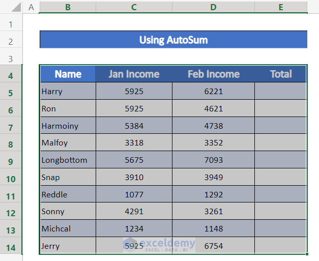
- Insert tab, select Tables > Table. Or you can press ‘Ctrl+T’ on your keyboard to create this table.
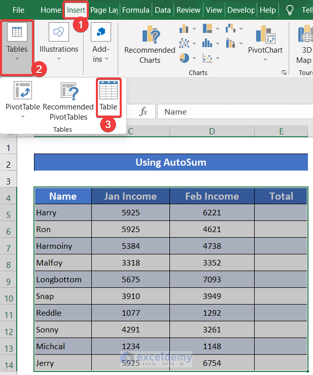
- A small dialog box entitled Create Table will appear.
- Click My Table has headers and OK at the bottom of that box.

- The Table will be created. We set the Table name ‘Income_1’ from the Table Design tab.
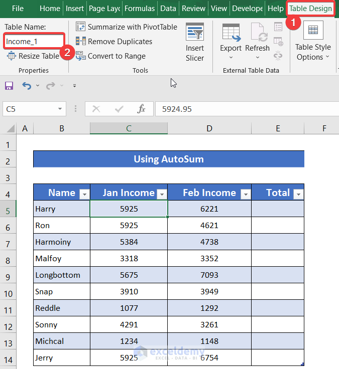
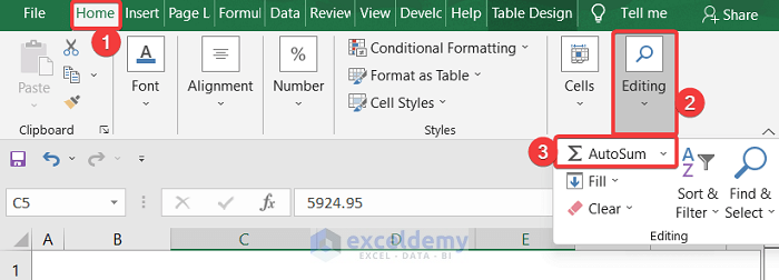
- Select the range of cells C5:E5.
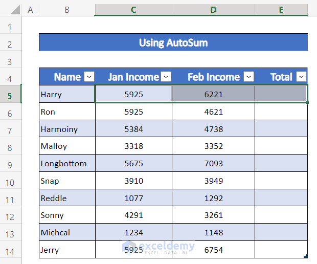
- In the Home ribbon, go to the Editing option.
- Select AutoSum.
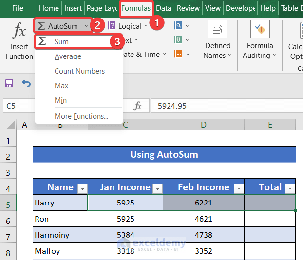
- Find this tool in the Formula in the Formula tab, select AutoSum > Sum.
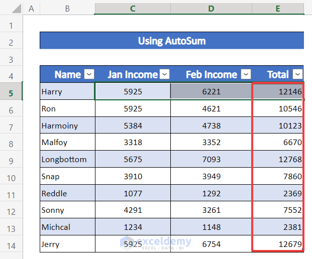
- You will get the result.
Method 2 – Keyboard Shortcut to Sum Columns
Steps:
- Select the entire range of cells to convert the datasheet into an Excel Table. We set the Table name ‘Income_2’ from the Table Design tab.
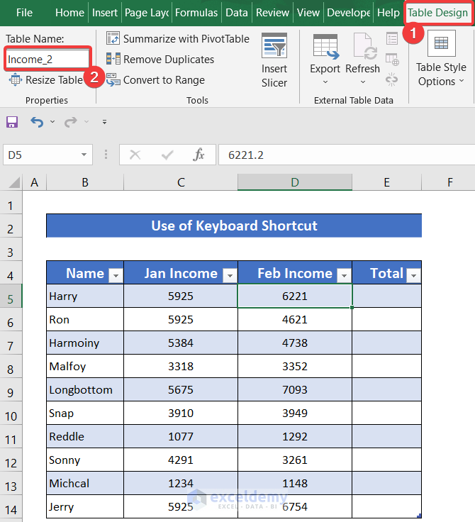
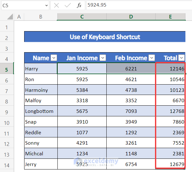
- After creating the table, select the range of cells C5:E5.

- Press ‘Alt+=’ on your keyboard.
- You will get the sum of Columns C and D row-wise in the column titles Total.
Method 3 – Using SUM Function
Steps:
- Select the entire range of cells to convert the datasheet into an Excel Table. It will provide us with more facilities. We set the table name as ‘Income’ from the Table Design ribbon.
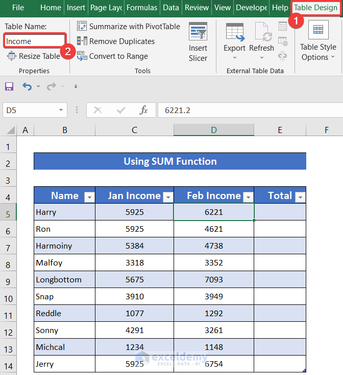
- Select cell E5.
- Write down the following formula into the cell.
=SUM(Income[@[Jan Income]:[Feb Income]])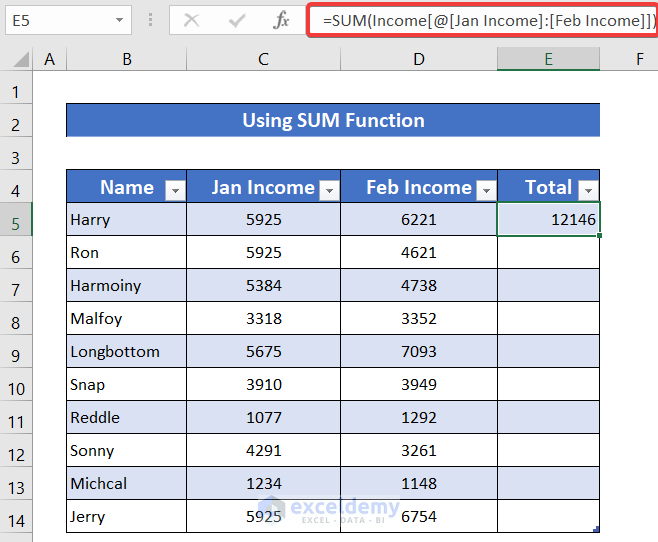
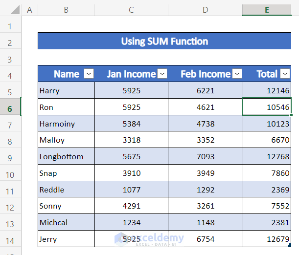
- Enter key on your keyboard to get the result.
Method 4 – SUBTOTAL Function to Sum Columns
Steps:
- Select the entire range of cells for converting the datasheet into an Excel Table. Set the table name as ‘Income_5’ from the Table Design tab.
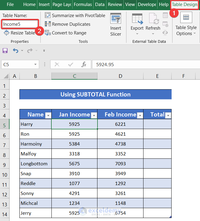
- Select cell E5 and write down the following formula for the cell.
=SUBTOTAL(9,Income5[@[Jan Income]:[Feb Income]])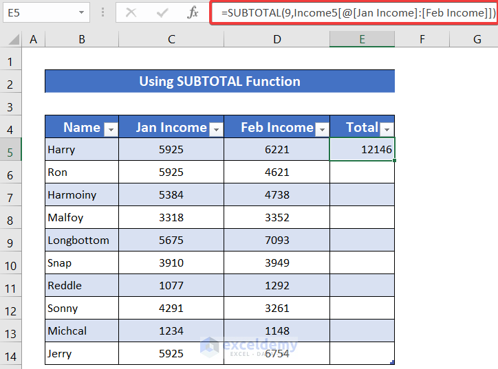
- Press Enter and you will get the result for all of the rows.
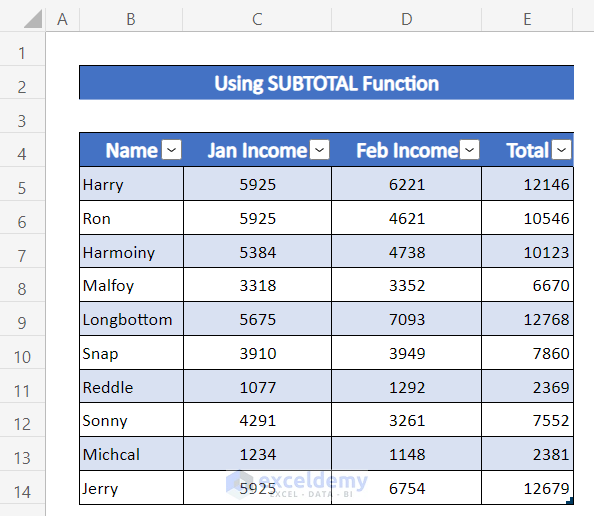
Method 5 – Applying AGGREGATE Function in Excel Table
Steps:
- Select the entire range of cells and convert the datasheet into an Excel Table. We set the table name as ‘Income56’ from the Table Design tab.
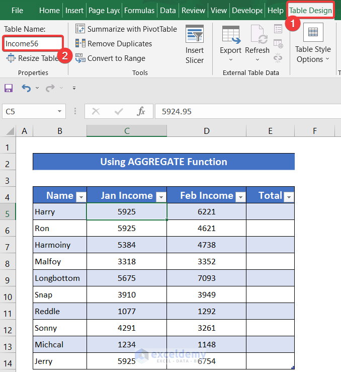
- Select cell E5 and write down the following formula for the cell.
=AGGREGATE(9,3,Income56[@[Jan Income]:[Feb Income]])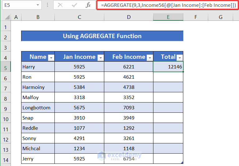
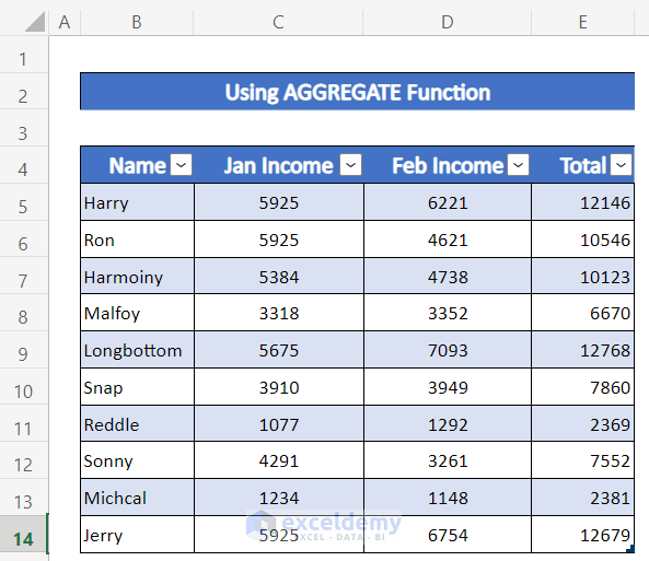
- Press Enter on your keyboard and you will get the result for all the rows.
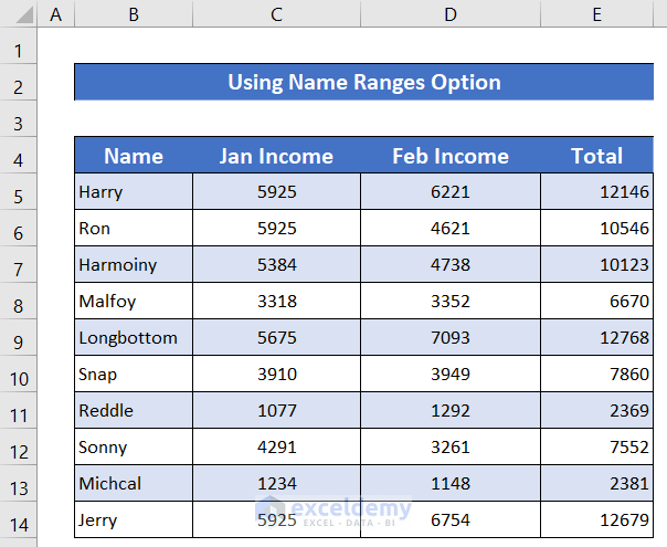
Method 6 – Defining Name Range to Add Columns in Excel
Steps:
- Select the range of cells C5:D5.
- Write down the range name in the box that shows us the active cell number.
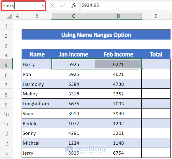
- We chose the employee name Harry as the range name.
- Press Enter on your keyboard.
- Define the name range for the rest of the rows.
- Select cell E5 and write down the following formula for the cell.
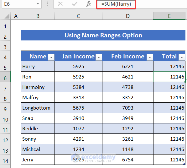
=SUM(Harry)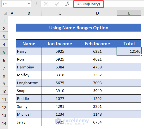
- Press Enter to get the sum into the cell.
- Write down the formula similar for the rest of the row to add them.
Things You Should Know
In this method, you should not convert the range of cells into an Excel Table. Because it will create trouble for you. You have seen in other methods, that when we write down the formula in cell E5 of the Excel table to sum the columns, it copies the sum formula for the other rows of column E. The Excel table will copy the formula ‘SUM(Harry)’ to the rest of the rows, instead of their own Defined Name. All the rows of this column will show the same result.
Method 7 – Sum Columns of Multiple Excel Tables
Steps:
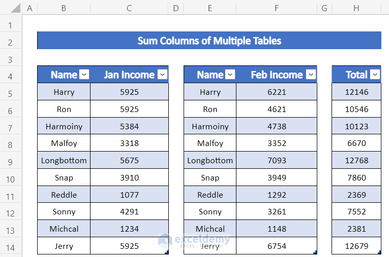
- Select the range of cells B5:C14, E5:F14, and H5:H14 to convert them into 3 different tables. We converted the column titled Total into a single table not to use the Fill Handle. We set the table’s name from the Table Design tab like the previous methods.
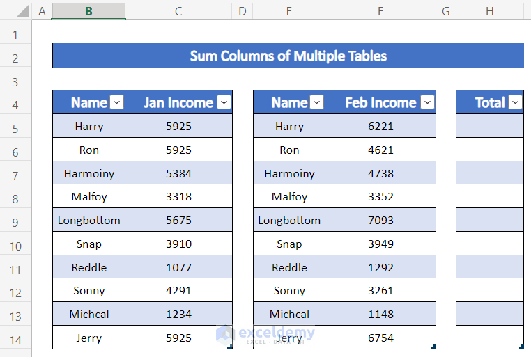
- Select cell H5.
- Write down the following formula in the cell.
=SUM(Income567[@[Jan Income]],Table8[@[Feb Income]])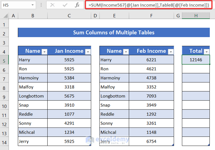
- Press the Enter key on your keyboard.
- You will get the sum of both columns for every row.
Download Practice Workbook
Download this practice workbook for practice while you are reading this article.
Related Articles
- How to Calculate Total Row and Column in Excel
- How to Sum Every Nth Column in Excel
- How to Sum Multiple Rows and Columns in Excel
<< Go Back to Sum Columns | Sum in Excel | Calculate in Excel | Learn Excel
Get FREE Advanced Excel Exercises with Solutions!


