Download the Practice Workbook
4 Quick Ways to Sum Multiple Rows in Excel
Method 1 – Using the SUM Function in Excel
Case 1.1 – Sum Multiple Rows into a Single Cell
In the following example, there are some numbers of products that are in stock in January and February. We want to sum up the numbers of product rows in a single cell.
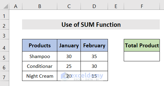
Steps:
- Select the cell where you want to put the result.
- Insert the following formula:
=SUM(C5:D7)- Press Enter.
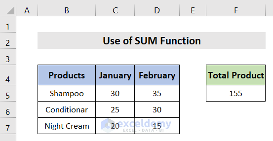
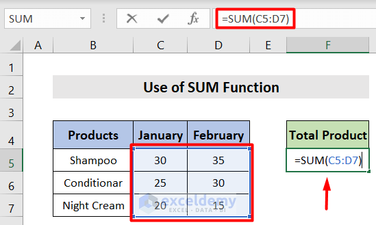 The sum of those three rows is shown in a single cell.
Case 1.2 – By Selecting the Entire Row as Reference
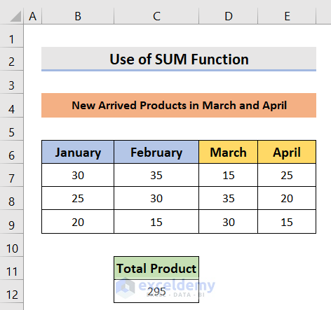
Assume that new products arrive in March and April. We need to sum those products by just selecting the row numbers.
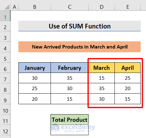
Steps:
- Select a cell and use the formula:
=SUM(7:9)- Hit Enter.
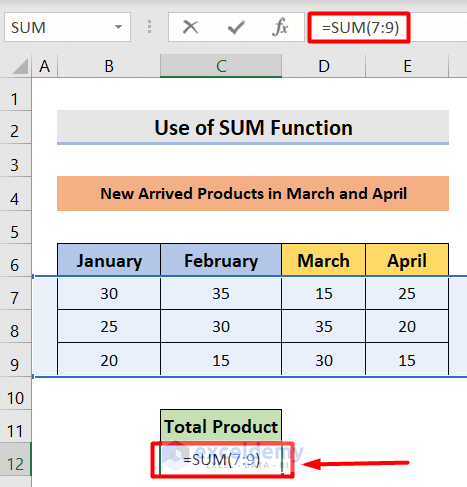
- This will add multiple rows of numbers together to get the total number in those rows.
Read More: How to Sum Selected Cells in Excel (4 Easy Methods)
Method 2 – AutoSum Multiple Rows
Case 2.1 – AutoSum Feature
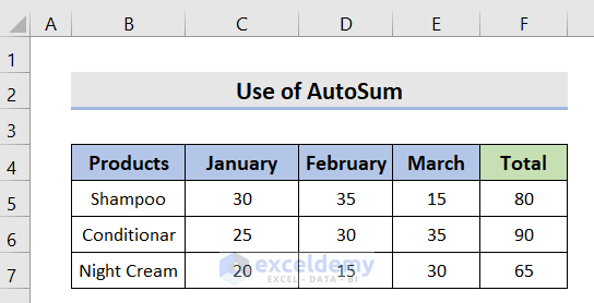
We need to sum the total of each product in the rows.
Steps:
- Select the cells with the data and the blank cells.
- Go to the Formula tab and choose AutoSum.
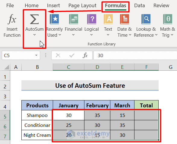
- Each of the rows will sum up automatically.
Case 2.2 – AutoSum Keyboard Shortcut
Steps:
- Select the dataset and press the Alt + = keys simultaneously.
- This adds the sum below the cells.
Read More: Sum Formula Shortcuts in Excel (3 Quick Ways)
Similar Readings
- How to Sum by Group in Excel (4 Methods)
- [Fixed!] Excel SUM Formula Is Not Working and Returns 0 (3 Solutions)
- How to Sum Only Visible Cells in Excel (4 Quick Ways)
- 3 Easy Ways to Sum Top n Values in Excel
- How to Sum Only Positive Numbers in Excel (4 Simple Ways)
Method 3 – Using the SUMPRODUCT Function in Excel
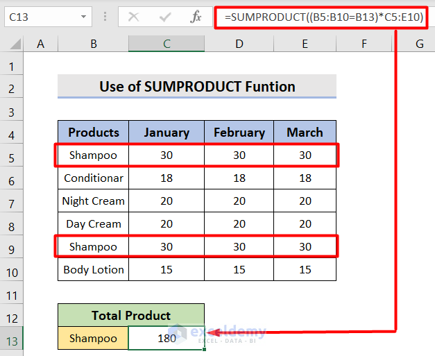
Let’s sum the duplicate products in row 5 and row 9.
Steps:
- Select the result cell.
- Insert the following formula:
=SUMPRODUCT((B5:B10=B13)*C5:E10)- Press Enter to see the result.
Read More: How to Add Multiple Cells in Excel (6 Methods)
Method 4 – Sum Matching Values from Multiple Rows in Excel
In the following example, there are three teams. We have to sum each team’s total goals.
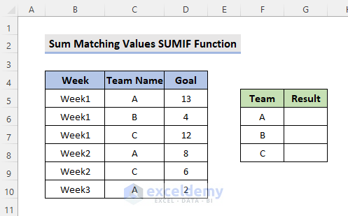
Steps:
- Select the cell for team A.
- Insert the following formula:
=SUMIF(C5:C10,"A",D5:D10) - Use the following formula for team B:
=SUMIF(C5:C10,"B",D5:D10) - Use the following for team C:
=SUMIF(C5:C10,"C",D5:D10) 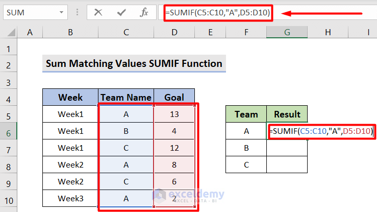
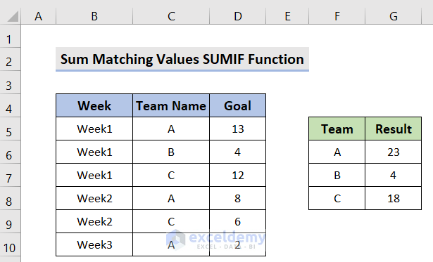
- The total goals of each team will be shown in the result column.
Read More: Excel Sum Last 5 Values in Row (Formula + VBA Code)
Related Articles
- Calculate Cumulative Sum in Excel (9 Methods)
- How to Calculate Sum of Squares in Excel (6 Quick Tricks)
- Sum Columns in Excel (7 Methods)
- How to Sum Between Two Numbers Formula in Excel
- Sum Cells in Excel: Continuous, Random, With Criteria, etc.
- How to Sum Multiple Rows and Columns in Excel


