This is an overview of the method and the sample dataset.
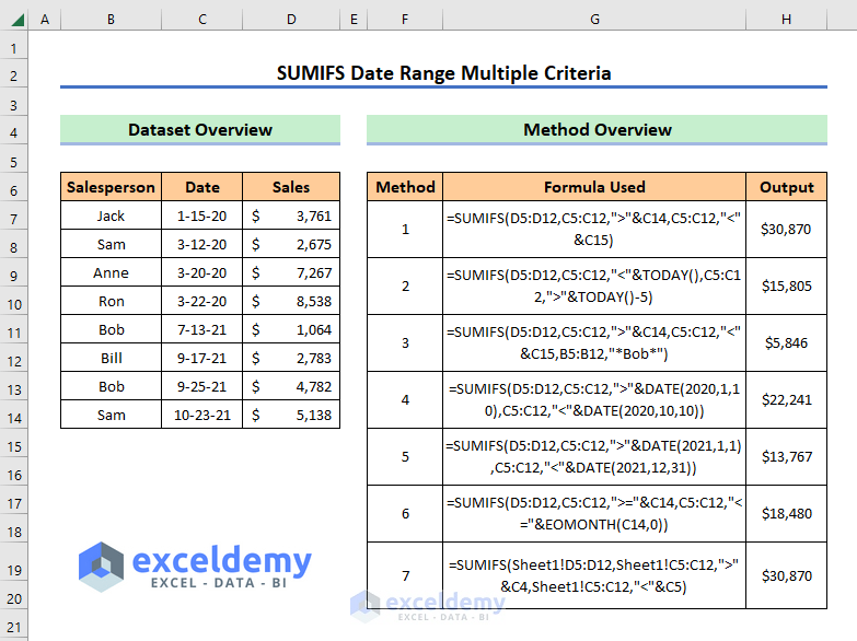
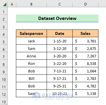
In this sample dataset you want to find the total sales over the dates.
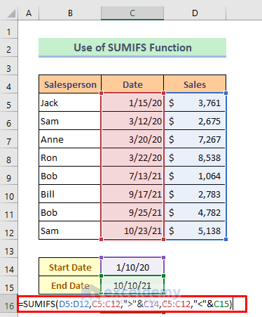
Method 1 – Using the SUMIFS Function to calculate a value Between Two Dates
Steps:
- Select C16
- Enter the formula below:
=SUMIFS(D5:D12,C5:C12,">"&C14,C5:C12,"<"&C15)- Press ENTER.
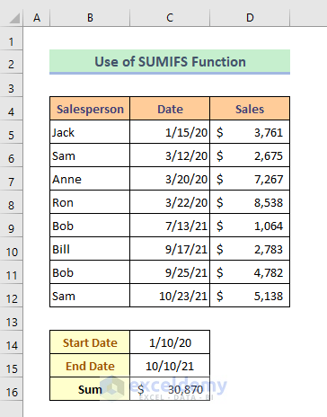
This is the output.
Method 2 – Combination of the SUMIFS and the TODAY Functions to Enter a Date Range with Criteria
Steps:
- Enter this formula in C14.
=SUMIFS(D5:D12,C5:C12,"<"&TODAY(),C5:C12,">"&TODAY()-5)- Press ENTER.
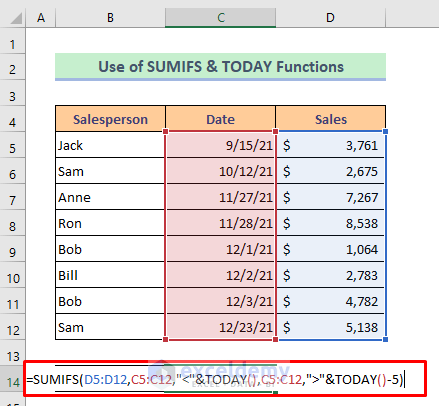
This is the output.
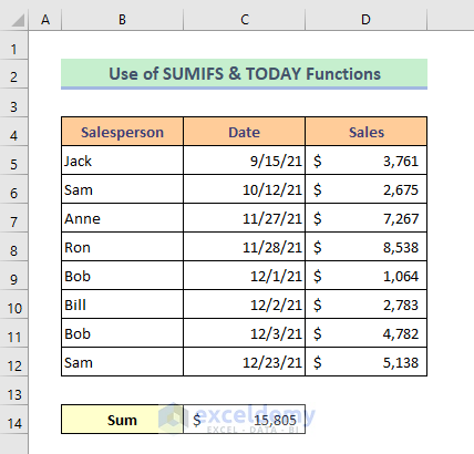
Formula Breakdown
TODAY() extracts todays’ date. It will return – {11/31/2021}
SUMIFS(D5:D12,C5:C12,”<“&TODAY(),C5:C12,”>”&TODAY()-5) calculates the sum between the date from the TODAY function and the 5 previous days. We subtracted 5 from the today function. That will result in –{15805}
Note: To calculate a sum between today and the 5 following days use +5 in the formula.
Method 3 – Using the SUMIFS Function to calculate a Sum Between Two Dates with Additional Criteria
Steps:
- Enter the formula in C16.
=SUMIFS(D5:D12,C5:C12,">"&C14,C5:C12,"<"&C15,B5:B12,"*Bob*")- Press ENTER.
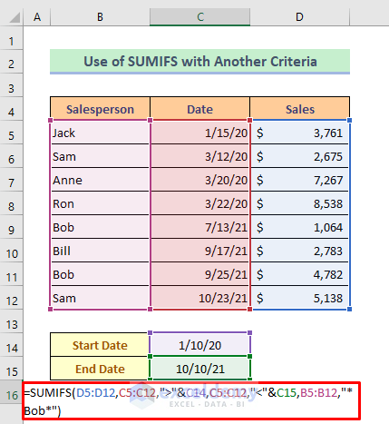
The sales value for Bob is calculated.
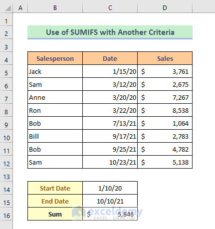
Method 4 – Using the SUMIFS and the DATE Functions Together to Sum with Multiple Criteria
Steps:
- Enter the formula in C16:
=SUMIFS(D5:D12,C5:C12,">"&DATE(2020,1,10),C5:C12,"<"&DATE(2020,10,10))- Press ENTER.
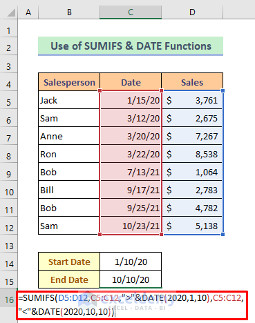
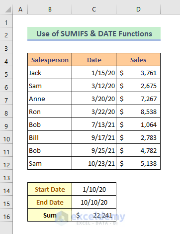
This is the output.
Formula Breakdown
The DATE function returns a serial number that corresponds to the given date. DATE(2020,1,10) returns-{43840} and DATE(2020,10,10) returns-{44114}.
➥ SUMIFS(D5:D12,C5:C12,”>”&DATE(2020,1,10),C5:C12,”<“&DATE(2020,10,10)) sums up the sales value according to the date range and returns –{22241}
Method 5 – Inserting the SUMIFS and the DATE Functions to Sum in a Specific Year
Steps:
- Enter this formula in C16.
=SUMIFS(D5:D12,C5:C12,">"&DATE(2021,1,1),C5:C12,"<"&DATE(2021,12,31))- Press ENTER.
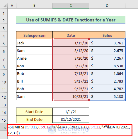
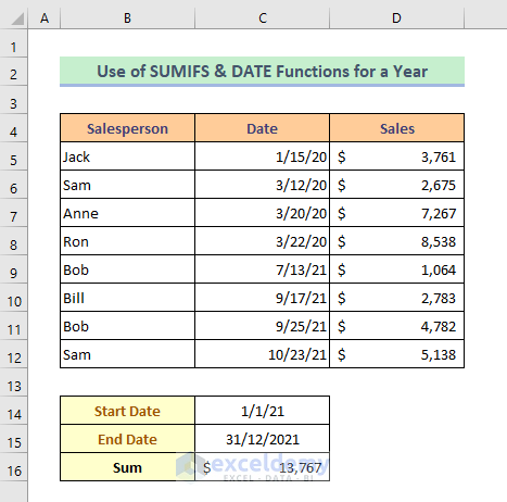
This is the output.
Method 6 – Combining the SUMIFS and EOMONTH Functions to Sum in a Specific Month
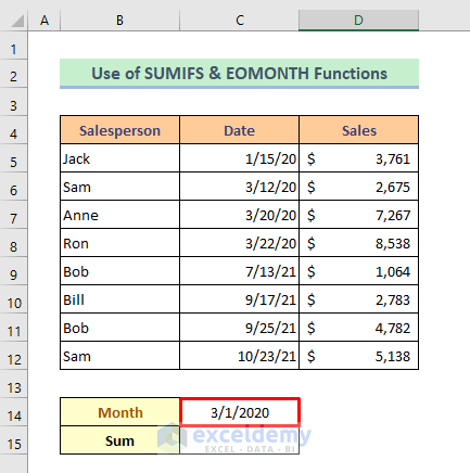
Step 1:
- Enter the first date of March in C14
Step 2:
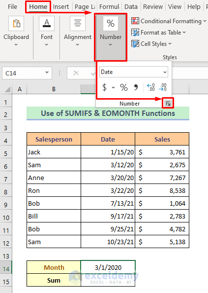
- Select that cell and click Home > Number > Arrow icon.
The dialog box “Format Cells” will open.
Step 3:
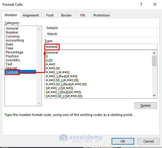
- Choose Custom.
- Enter “mmmm” in Type.
- Click Ok.
The cell will show the name of the month.
Step 4:
- Enter this formula in C15.
=SUMIFS(D5:D12,C5:C12,">="&C14,C5:C12,"<="&EOMONTH(C14,0))- Press ENTER.
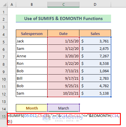
This is the output.
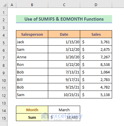
Formula Breakdown
➥ EOMONTH(C14,0) stores the date as a sequential serial number so it can be used in the calculation. It will return {43921}
➥ SUMIFS(D5:D12,C5:C12,”>=”&C14,C5:C12,”<=”&EOMONTH(C14,0)) calculates the sales value according to the date range and returns {18480}
Method 7- Using the SUMIFS Function to calculate a Sum Between a Date Range from Another Sheet
This is “Sheet1”.
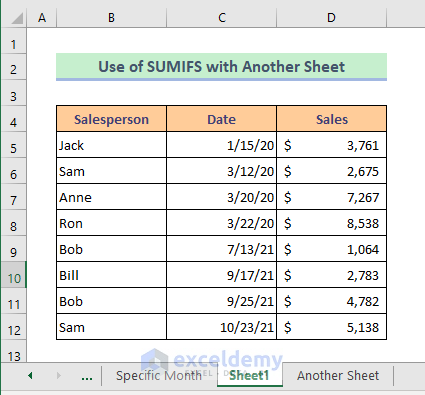
“Another Sheet” will be used to calculate.
Steps:
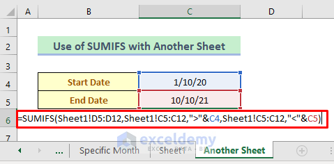
- Enter this formula in C6 .
=SUMIFS(Sheet1!D5:D12,Sheet1!C5:C12,">"&C4,Sheet1!C5:C12,"<"&C5)- Press ENTER.
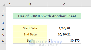
This is the output.
Download Practice Book
Download the free Excel template here to practice.
Related Article
<< Go Back to SUMIFS with Date Range | Excel SUMIFS Function | Excel Functions | Learn Excel
Get FREE Advanced Excel Exercises with Solutions!


This is very helpful. I just have one question. When I try to do a sumifs with date ranges, I only get 0s. I figured out that it must be because I have a lot of data points with the same date. My rows are employees’ voids. I pulled the data for last year. Obviously, a lot of voids happen on a single date. I changed the dates to make them all different (even by just a day), and it works. What do I need to do to use this sumifs function for my purposes. Thank you
Greetings, Nat Troy. We don’t have a large enough dataset to test your problem. Please send us your file to [email protected]. So we can take a closer look at the issue.