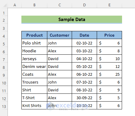
We’ll use a dataset that has the Product, Customer, Date, and Price for different sales.
Method 1 – Apply SUMIFS with Multiple Criteria Vertically
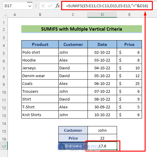
- Insert the criteria for the customer in D15 and the price in D16.
- Go to cell D17 and apply the following formula:
=SUMIFS(E5:E13,C5:C13,D15,E5:E13,"<"&D16)- sum_range=E5:E13 or Price column
- criteria _range1=C5:C13 or Customer column
- criteria1=D15. This argument will find the name of the customer named John in row 5,10,13
- criteria _range2=E5:E13 or Price column
- criteria2=“<“&D16. This argument will find a value that is less than 22 in the range of E5:E13
- Hit the Enter button. You’ll get the sum of all values that conform to the criteria.
Read More: How to Use SUMIFS with Multiple Criteria in the Same Column
Method 2 – Combine Other Excel Functions with SUMIFS to Match Multiple Horizontal and Vertical Criteria
Case 2.1 – Combining SUMIFS, OFFSET, MATCH, and COUNT Functions
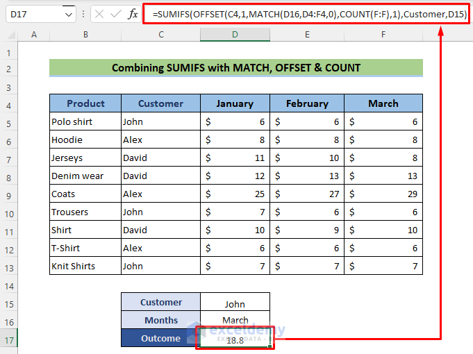
We will add all the price values for John that are in the month of March.
- Insert the following formula in cell D17:
=SUMIFS(OFFSET(C4,1,MATCH(D16,D4:F4,0),COUNT(F:F),1),Customer,D15)- sum_range=OFFSET(C4,1,MATCH(D16,D4:F4,0),COUNT(F:F),1)
- criteria _range1= Customer column
- criteria1=D15 or March
- Hit the Enter button.
Read More: How to Apply SUMIFS with Multiple Criteria in Different Columns
Case 2.2 – Combining INDEX-MATCH with SUMIFS
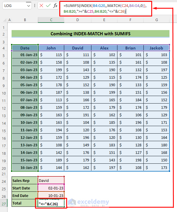
We will add all the price values for David that are between 02/01/23 and 10/01/23.
- Go to cell D17 and apply the following formula:
=SUMIFS(INDEX(B4:G20,,MATCH(C24,B4:G4,0)),B4:B20,">="&C25,B4:B20,"<="&C26)Here,
- sum_range=INDEX(B4:G20,,MATCH(C24,B4:G4,0))
- criteria _range1= Customer column
- criteria1=D15 or March
- Hit the Enter button.
Read More: How to Apply SUMIFS with INDEX MATCH for Multiple Columns and Rows
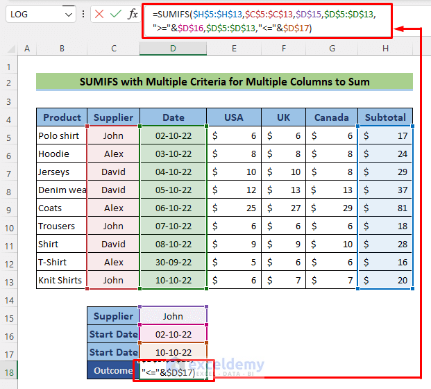
Method 3 – SUMIFS with Multiple Criteria for Multiple Columns to Sum
We will add all the price values for John between 02/10/22 and 10/10/22.
- Create a new subtotal column H that will sum the prices in the previous three columns.
- Go to cell D17 and apply the following formula:
=SUMIFS($H$5:$H$13,$C$5:$C$13,$D$15,$D$5:$D$13,">="&$D$16,$D$5:$D$13,"<="&$D$17)- sum_range=$H$5:$H$13
- criteria _range1= $C$5:$C$13 or Supplier
- criteria1=$D$15 or John
- criteria _range2= $C$5:$C$13 or Supplier
- criteria2=$D$15 or John
- Hit the Enter button.
The SUMPRODUCT Function: Alternative to SUMIFS for Simultaneous Vertical and Horizontal Criteria in Excel
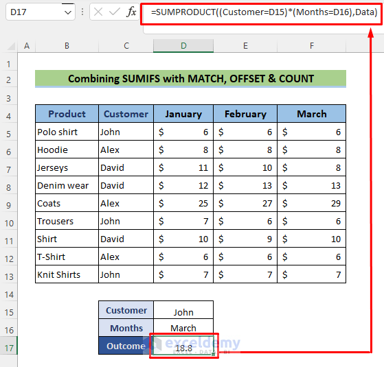
We will add all the price values for John that are in the month of March.
- Go to cell D17 and apply the following formula:
=SUMPRODUCT((Customer=D15)*(Months=D16),Data)Here,
- array1= (Customer=D15)*(Months=D16) creates an array {0,0,1;0,0,0;0,0,0;0,0,0;0,0,0;0,0,1;0,0,0;0,0,0;0,0,1}
- array1= Data creates an array {5.6,5.7,5.9;8.2,8.1,8.3;10.5,10.4,8.1;12.2,12.6,12.8;25,27,29;6.8,6.3,6.1;9.8,9.4,9.8;5.6,5.5,5.9;6.5,6.9,6.8}.
- SUMPRODUCT multiply this array that will have values: 5.9+6.1+6.8=18.8
- Hit the Enter button.
Read More: SUMIFS: Sum Range Across Multiple Columns
Download the Practice Workbook
Related Articles
- SUMIFS with Multiple Criteria Along Column and Row in Excel
- Exclude Multiple Criteria in Same Column with SUMIFS Function
- How to Use VBA Sumifs with Multiple Criteria in Same Column
<< Go Back to Excel SUMIFS with Multiple Criteria | Excel SUMIFS Function | Excel Functions | Learn Excel
Get FREE Advanced Excel Exercises with Solutions!

