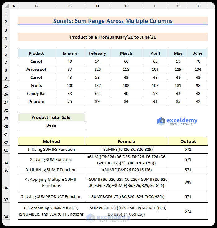
To demonstrate how to sum ranges, we have the following dataset of product sales for different months. Let’s determine the total number of sales for a specific product over the course of the month.
Method 1 – Using SUMIFS Function with Helper Column
Steps:
- Add a helper column I as Subtotal.
- Use the below formula in cell I6:
=SUM(C6:H6)
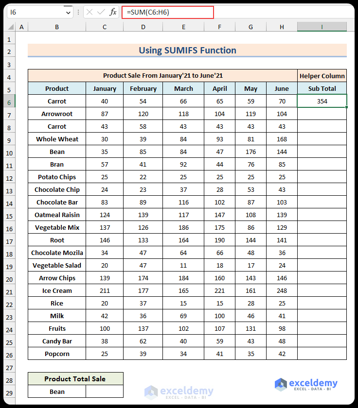
- Press Enter and then drag the Fill Handle down to the rest of column I.
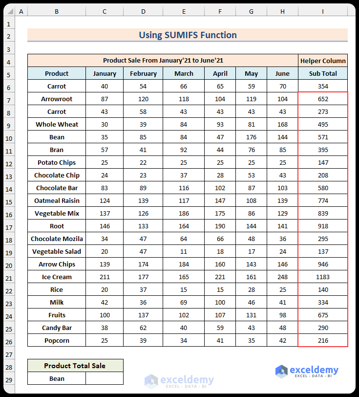
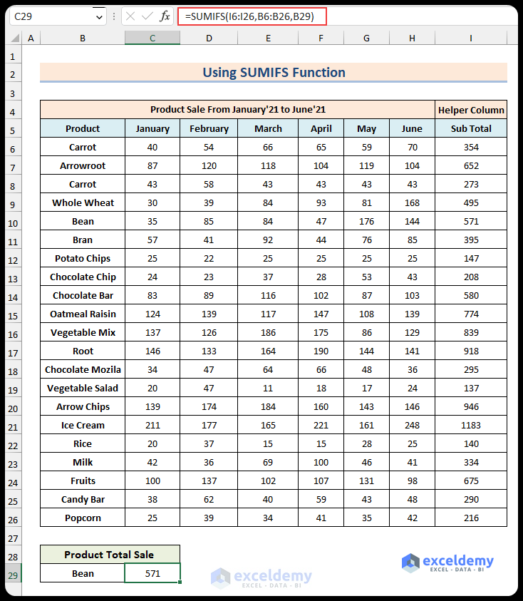
- Insert the following formula in cell C29 and hit Enter:
=SUMIFS(I6:I26,B6:B26,B29)
- The total Product Sale number of B29 (cell criteria Bean) will appear.
Read More: Excel SUMIFS with Multiple Vertical and Horizontal Criteria
Method 2 – Using the SUM Function
Steps:
- Insert the following formula in cell C29:
=SUM((C6:C26+D6:D26+E6:E26+F6:F26+G6:G26+H6:H26)*(--(B6:B26=B29)))
In the formula, (C6:C26+D6:D26+E6:E26+F6:F26+G6:G26+H6:H26) defines the sum of individual six ranges. Then, (B6:B26=B29) declares the range value to be equal to B29 (Bean).
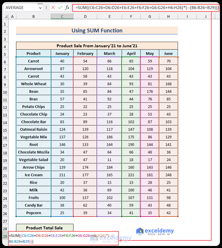
- Press Enter. For earlier versions of Excel, press Ctrl + Shift + Enter.
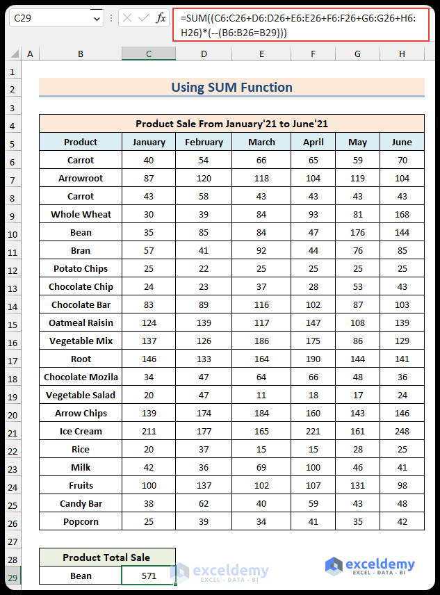
- You can use any name of the product in the B29 cell to count the total product sales.
Method 3 – Utilizing SUMIF Function
Steps:
- Add a helper column I (see Method 1)
- Type the following formula in cell C29.
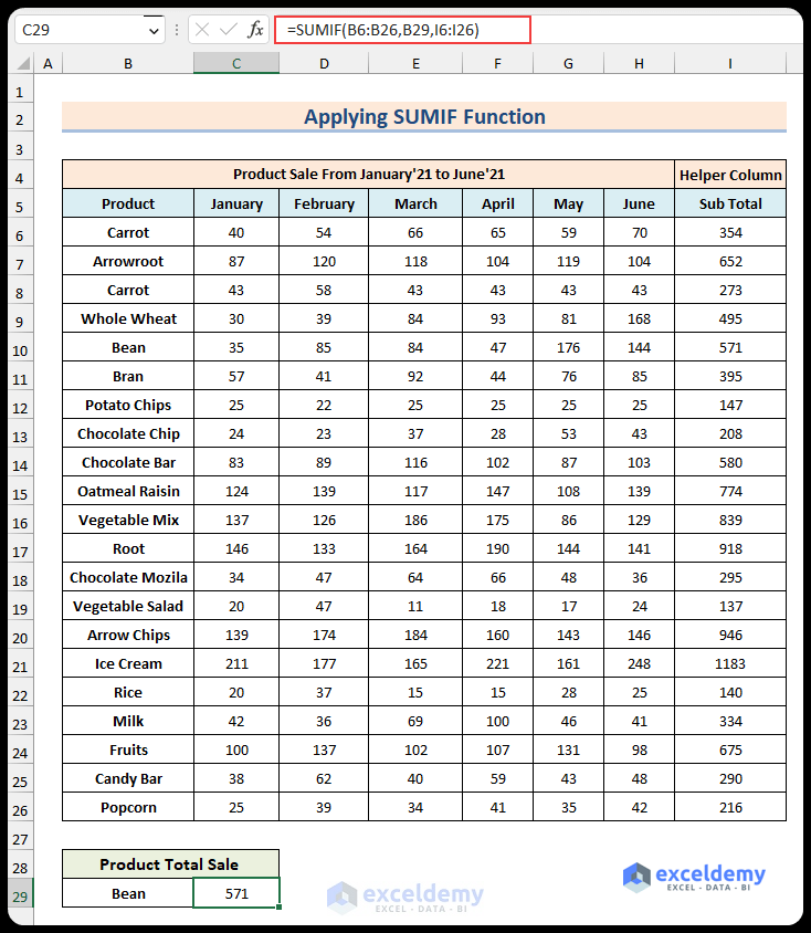
=SUMIF(B6:B26,B29,I6:I26)
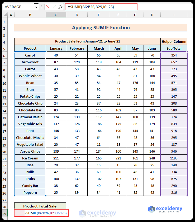
- Press Enter.
Read More: How to Use SUMIFS with Multiple Criteria in the Same Column
Method 4 – Applying Multiple SUMIF Functions
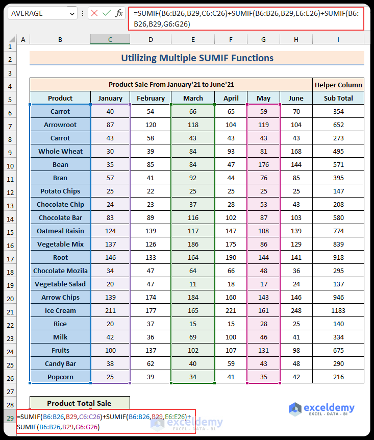
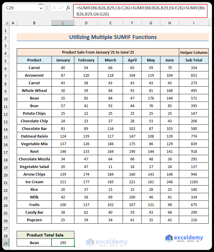
Let’s say we want to sum the product sales in random months such as January, March, and May.
Steps:
- Enter this formula in cell C29:
=SUMIF(B6:B26,B29,C6:C26)+SUMIF(B6:B26,B29,E6:E26)+SUMIF(B6:B26,B29,G6:G26)
- In the formula, SUMIF(B6:B26,B29,C6:C26); is a sum of product sales for B3 products in the B6:B26 range, passing the value to sum from the C6:C26 range. The other SUMIFS repeat the process for the remaining columns we need.
- Press Enter.
Read More: How to Apply SUMIFS with Multiple Criteria in Different Columns
Method 5 – Using SUMPRODUCT Function
Since we want the sum of the total sales of a particular product, we can use the product name as a ”text” reference.
Steps:
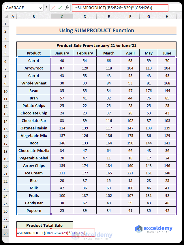
- Use the following formula in cell C29:
=SUMPRODUCT((B6:B26=B29)*(C6:H26))
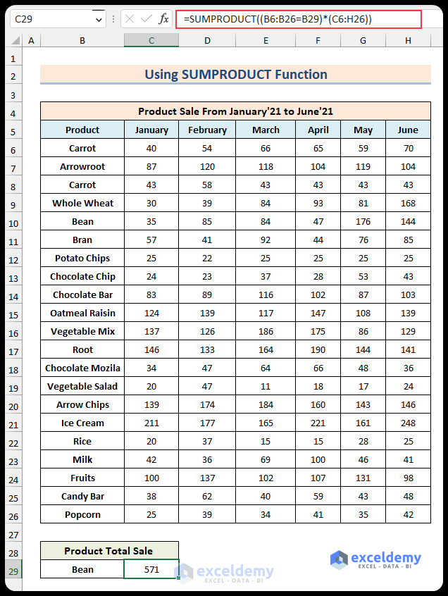
Inside the formula, (C6:H26); returns the criteria as True or False. (B6:B26=B29)*(C6:H26) multiplies the values with the criteria and outputs True or False. SUMPRODUCT((B6:B26=B29)*(C6:H26)) displays the total sale value.
- Press Enter and the total number of sales of the product “Bean” (listed in B29) will appear.
Read More: SUMIFS with Multiple Criteria Along Column and Row in Excel
Method 6 – Combining SUMPRODUCT, ISNUMBER, and SEARCH Functions
Consider that your initial dataset contains additional information in the Product box, so that it won’t always exactly match the search cell.
Steps:
- Copy the following formula in cell B29:
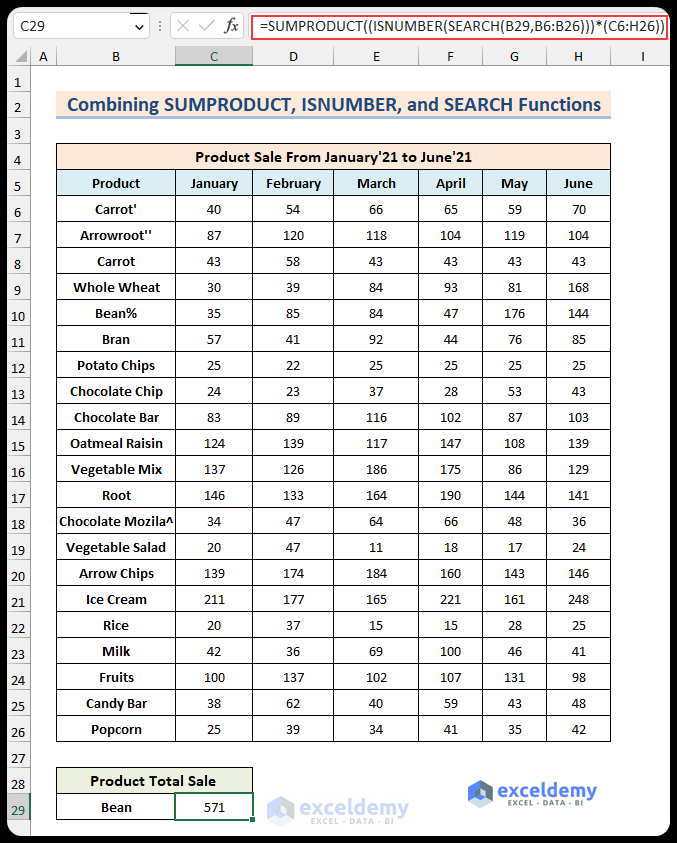
=SUMPRODUCT((ISNUMBER(SEARCH(B29,B6:B26)))*(C6:H26))
The formula works the same as described in Method 5, but the ISNUMBER and SEARCH functions ignore any additional text in product names.
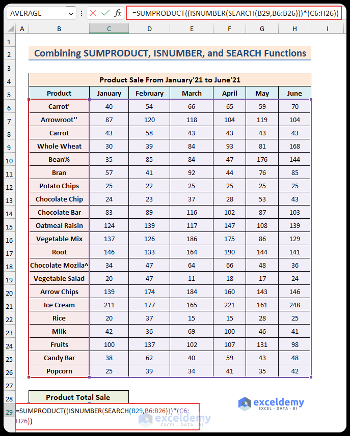
- Press Enter and the total sale number of “Bean” appears.
Download Practice Workbook
You can download the Excel file from the link below.
Related Articles
- How to Apply SUMIFS with INDEX MATCH for Multiple Columns and Rows
- Exclude Multiple Criteria in Same Column with SUMIFS Function
- How to Use VBA Sumifs with Multiple Criteria in Same Column
<< Go Back to Excel SUMIFS with Multiple Criteria | Excel SUMIFS Function | Excel Functions | Learn Excel
Get FREE Advanced Excel Exercises with Solutions!

