How to Use Excel SUMIFS with Multiple Criteria in Same Column

Here’s an overview of using the SUMIFS function to filter a table based on different criteria and options.

⏷Problem with Excel SUMIFS Function
⏷SUM and SUMIFS Functions with Multiple Criteria
⏷SUM and SUMIFS Functions with 3 Criteria
⏷SUM and SUMIFS Functions with Wildcards
⏷SUMIFS Function with Multiple Date Criteria
⏵Using a Specific Date
⏵Using Today’s Date
⏷Multiple SUMIFS Functions for Multiple OR Criteria
⏷Alternative: Using Multiple SUMIF Functions

Problem with Excel SUMIFS Function While Using Multiple Criteria in the Same Range of a Column

Here’s the syntax of the SUMIFS function:

SUMIFS(sum_range, criteria_range1, criteria1, [criteria_range2, criteria2], ...)

From the syntax, it should work for multiple criteria and criteria ranges.

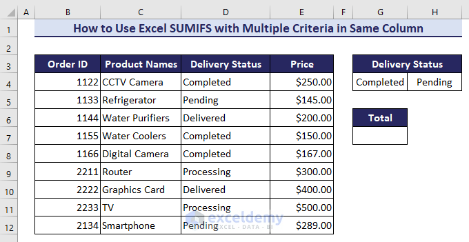
We took a dataset that contains some electronic products’ ID, delivery status, and price.

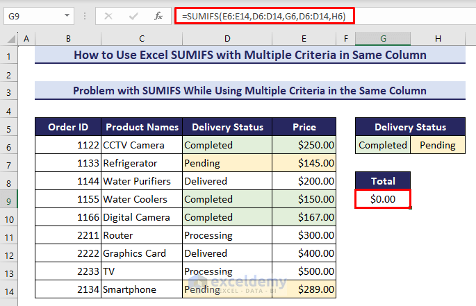
Insert the following formula in cell G9 and hit the Enter button to calculate the total price of the products with ‘Completed’ and ‘Pending’ status:

=SUMIFS(E6:E14,D6:D14,G6,D6:D14,H6)

Unfortunately, it returned zero! The SUMIFS function only works for AND criteria with different columns, not for OR criteria in the same column. So as we applied the same criteria range separately, the SUMIFS function returned zero.

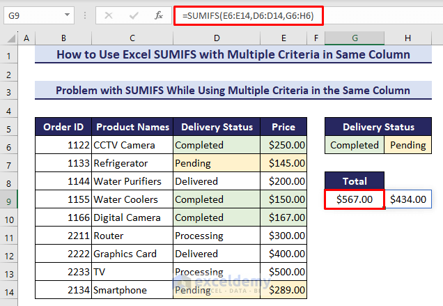
Here’s an example where the SUMIFS function returned the result separately as an array:

=SUMIFS(E6:E14,D6:D14,H5:I5)

But we expect the output just in a cell.

Example 1 – Combining SUM and SUMIFS Functions with Multiple Criteria in Same Column

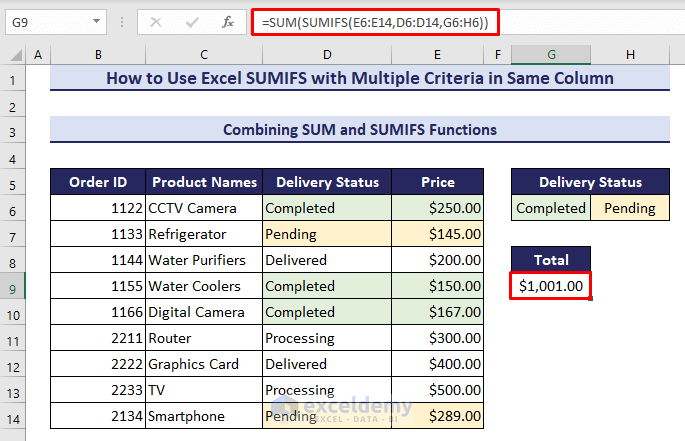
Apply the following formula in cell G9 to get the total price:

=SUM(SUMIFS(E6:E14,D6:D14,G6:H6))

You can also use the SUMPRODUCT function instead of the SUM function, it will give you the same result.

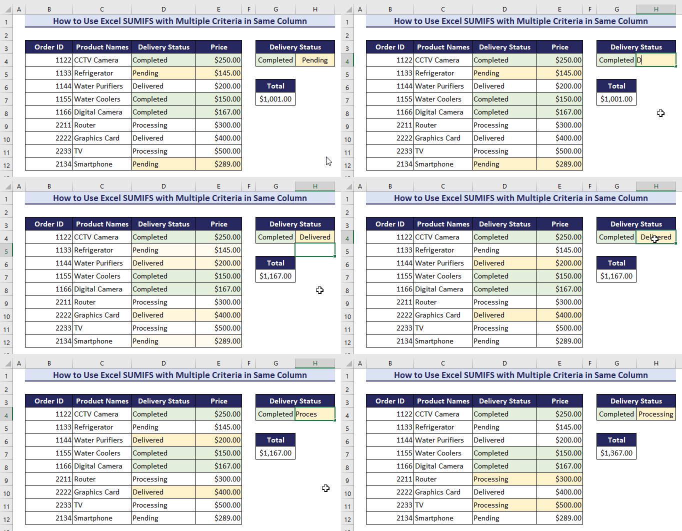
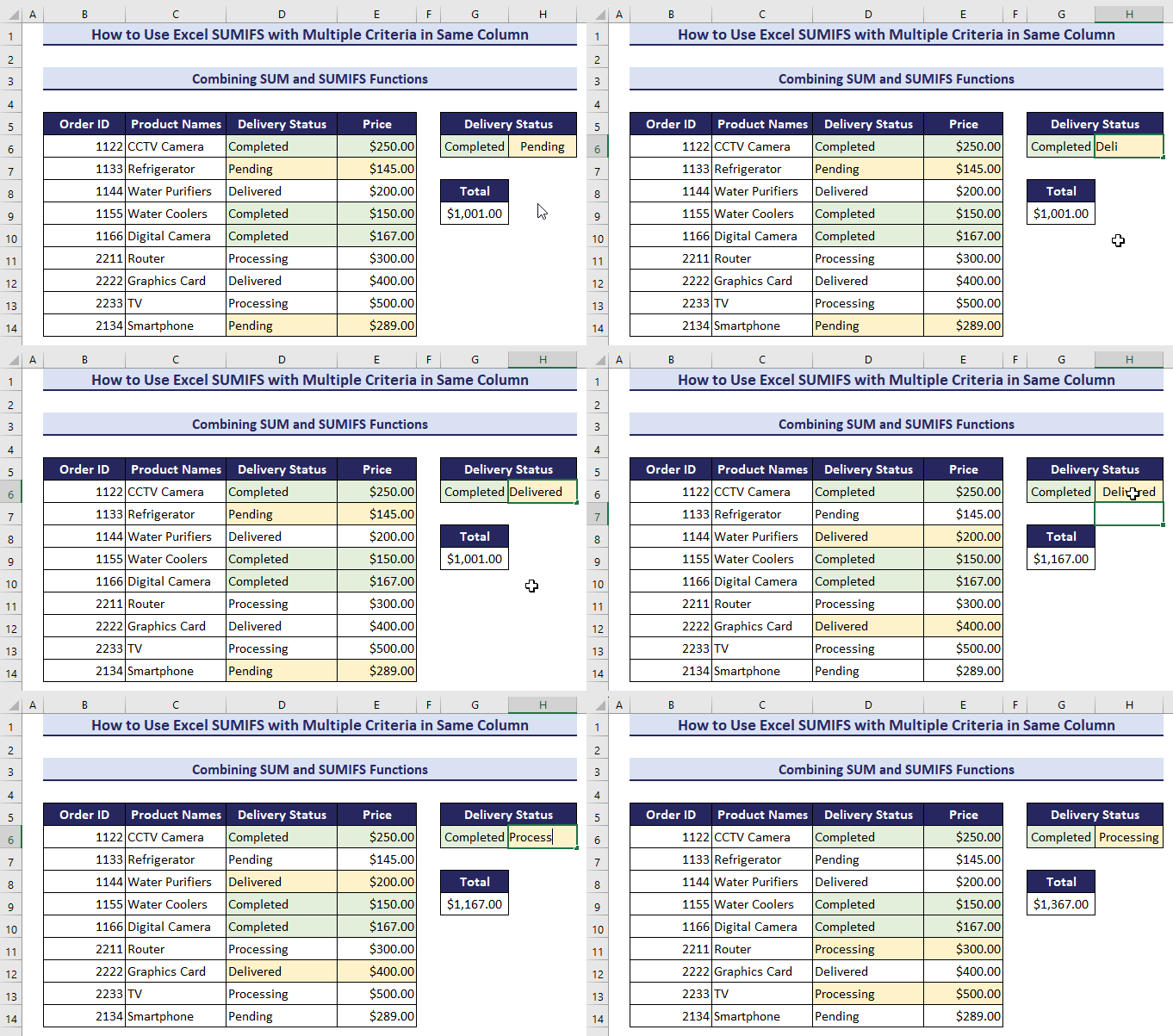
The corresponding data in the dataset will be highlighted instantly whenever you change the criteria.

Note:

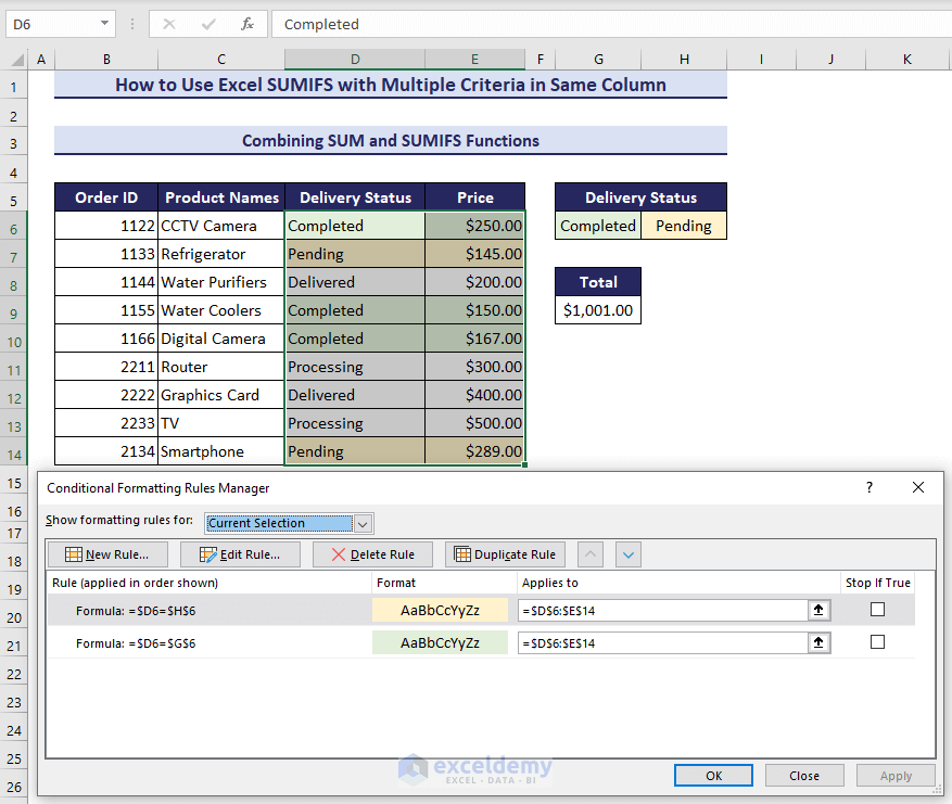
We used conditional formatting to highlight different matched criteria.

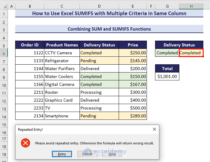
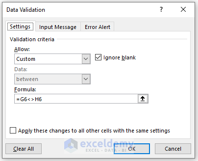
We applied data validation rules to restrict the repeated entry of the criteria. Otherwise, the SUMIFS function will return the wrong result.

Here’s the formula we used as validation criteria:

Example 2 – Joining SUM and SUMIFS Functions with 3 Criteria in Same Column

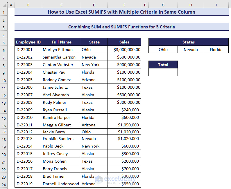
We’ll expand the array criteria in the SUMIFS function. For the below dataset, we’ll calculate the total sales for three states: Ohio, Nevada, and Florida.

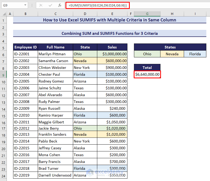
In cell G9, insert the following formula and press the Enter button:

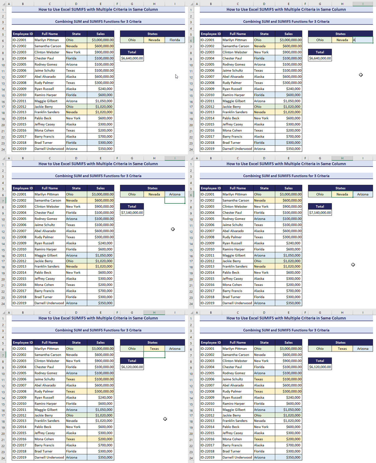
=SUM(SUMIFS(E6:E24,D6:D24,G6:I6))

See the below GIF to get a complete overview.

Example 3 – Combining SUM and SUMIFS Functions with Wildcards for Partial Match

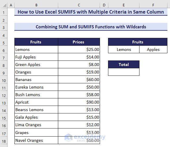
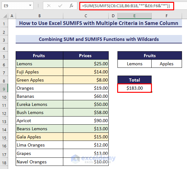
We’ll take a new dataset that has different types of Fruits and their corresponding Prices. Some fruits have different types of species, such as Eureka Lemons, Bush Lemons, and Bearss Lemons. We’ll use a formula that will sum the prices if it gets the partial text ‘Lemons’ and ‘Apples’ in any corresponding cell.

Insert the following formula in cell E9 and hit the Enter button:

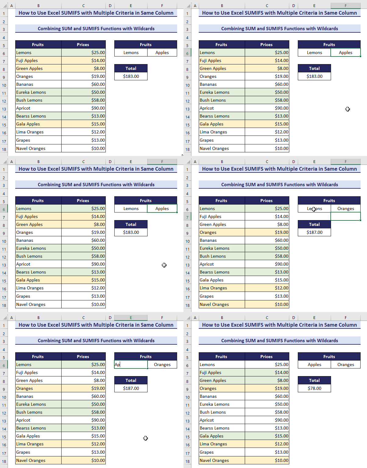
=SUM(SUMIFS(C6:C18,B6:B18,"*"&E6:F6&"*"))

The formula recalculates and changes the highlighted cells whenever we change the criteria.

Example 4 – Using the SUMIFS Function with Multiple Date Criteria in the Same Column

Case 4.1 – Using a Specific Date

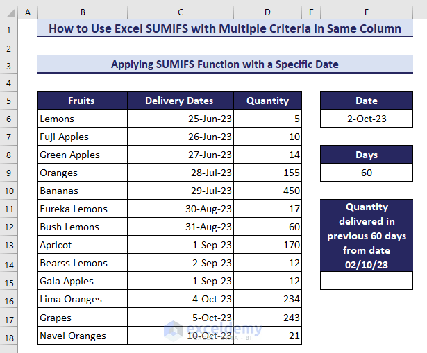
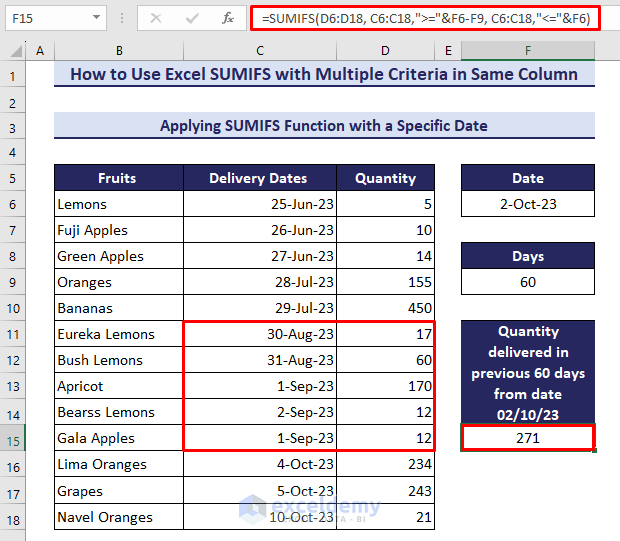
Let’s calculate the delivered quantity within the previous 60 days from the date ‘2-Oct-23’ for the below dataset.

Use the following formula in cell F15:

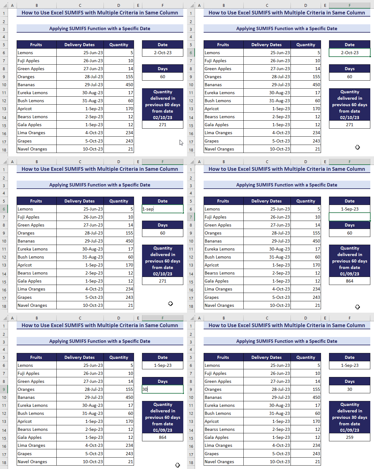
=SUMIFS(D6:D18, C6:C18,">="&F6-F9, C6:C18,"<="&F6)

If you update the date and number of days, the formula will show the quantity according to that. The output header will also be updated.

Case 4.2 – Using Today’s Date

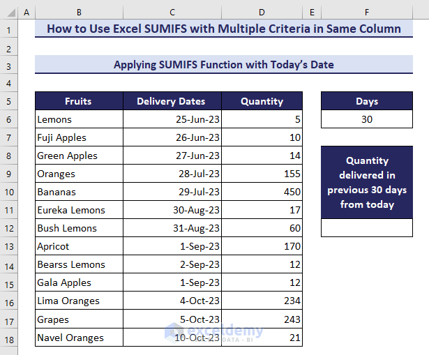
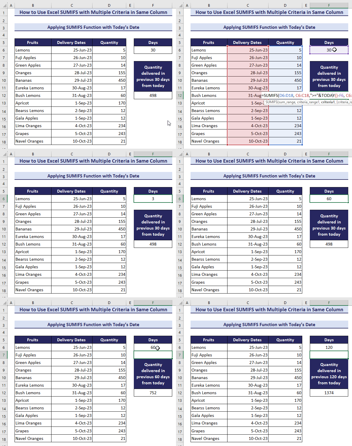
If we use the TODAY function instead of the fixed date, then it will calculate the delivered quantity within the previous 30 days from today’s date.

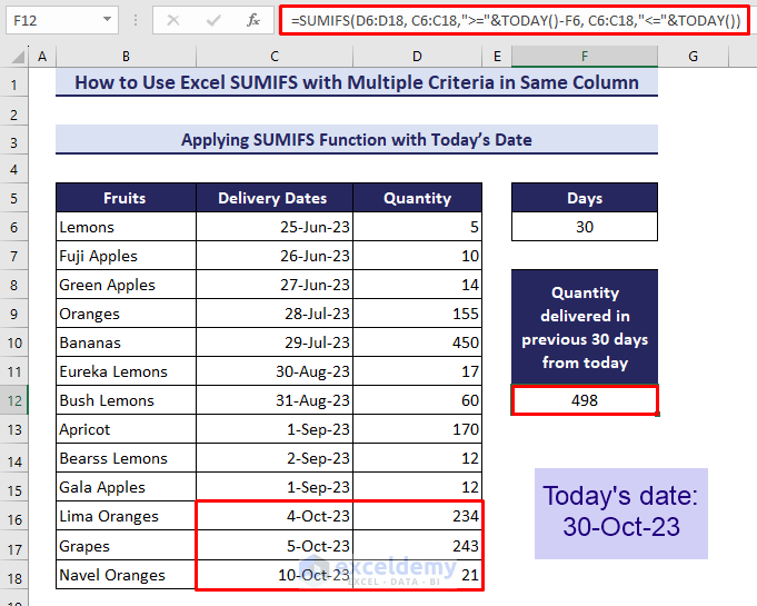
In cell F12, apply the following formula and press Enter:

=SUMIFS(D6:D18, C6:C18,">="&TODAY()-F6, C6:C18,"<="&TODAY())

Today’s date is 30-Oct-23 as of time of writing, so the formula is returning the delivered quantity within 30 days from 30-Oct-23.

If you update the number of days, it will update the delivered quantity from today for that number of days.

Example 5 – Joining Multiple SUMIFS Functions for Multiple OR Criteria

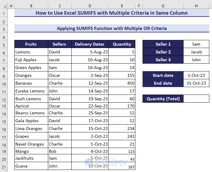
We added a new column in our previous dataset, which represents seller’s names. Let’s calculate the total delivered quantity for three sellers within a date range.

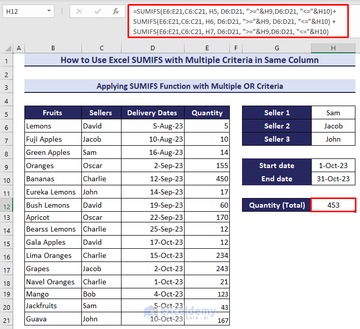
Insert the below formula in cell H12:

=SUMIFS(E6:E21,C6:C21, H5, D6:D21, ">="&H9,D6:D21, "<="&H10)+SUMIFS(E6:E21,C6:C21, H6, D6:D21, ">="&H9, D6:D21, "<="&H10) +SUMIFS(E6:E21,C6:C21, H7, D6:D21, ">="&H9,D6:D21, "<="&H10)

After pressing the Enter button, it will return the summed quantity for the date range.

Using Multiple SUMIF Functions Instead of Excel SUMIFS with Multiple Criteria in Same Column

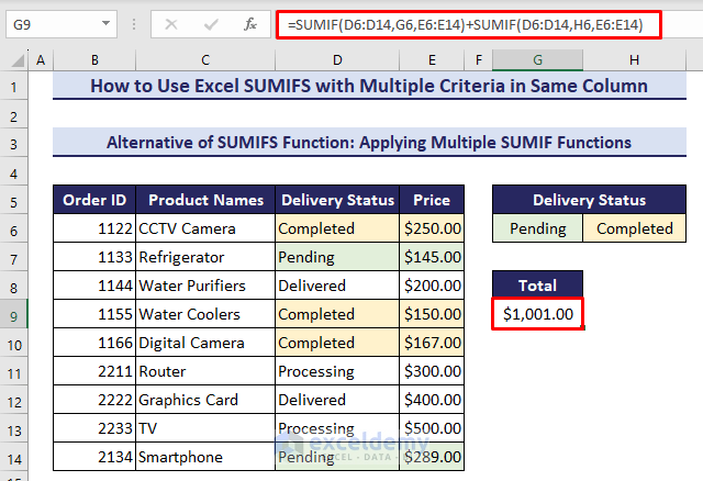
Use the following formula in cell G9 to calculate the total price for pending and delivered items:

=SUMIF(D6:D14,G6,E6:E14)+SUMIF(D6:D14,H6,E6:E14)

We got the same output as example 1.

Download the Practice Workbook

SUMIFS with Multiple Criteria in Same Column.xlsx

<< Go Back to Excel SUMIFS with Multiple Criteria | Excel SUMIFS Function | Excel Functions | Learn Excel

Get FREE Advanced Excel Exercises with Solutions!

2 Comments

Will Dec 3, 2021 at 3:26 AM

Hey Abdullah,

Helpful article; thanks for sharing. I am trying to sumifs using a date range, as you show above, but instead of having to type the starting date into the formula, I want to point at a cell that contains the date and then set rules off of that.

as an example, here is your formula above.

=SUMIFS(D4:D12, C4:C12,”>=”&TODAY()-60, C4:C12,”=”&Z13()-60, C4:C12,”<="&Z13())

Is something like that possible???
- Reply
  Tanjim Reza Aug 30, 2022 at 4:04 PM
  Hi, WILL!
  Thank you for your query!
  You can definitely point to a cell containing the desired date rather than typing it inside the formula. Say, you have placed the required date in the C15 cell.
  In that case, you can use the following formula:
```
=SUMIFS(D4:D12, C4:C12,">="&$C$15-60, C4:C12,"<="&$C$15)
```