Introduction to TEXTJOIN Function in Excel
Summary
- Concatenates a list or range of text strings into a single string using a delimiter.
- Can include both empty cells and non-empty cells.
- Available from Excel 2019.
Syntax
The syntax of the TEXTJOIN functions is:
=TEXTJOIN(delimiter,ignore_empty,text1,...)
Arguments Explanation
| Arguments | Required/Optional | Explanation |
|---|---|---|
| delimiter | Required | The delimiter by which the concatenated texts will be separated. |
| ignore_empty | Required | Tells whether to ignore the empty cells in the range or not. |
| text1 | Required | The first text string to be joined. |
| [text2] | Optional | The second text string is to be joined. |
| … | … | … |
| … | … | … |
- You can use a maximum number of 252 texts to join, like text1, text2, …, etc. up to text252.
- The text1, text2, …, etc arguments can be numbers also. Not necessary that they must be strings. The TEXTJOIN function can join numbers too.
Return Value
Returns a text string by joining all the given texts separated by the delimiter.
How to Use TEXTJOIN Function in Excel: 7 Suitable Examples
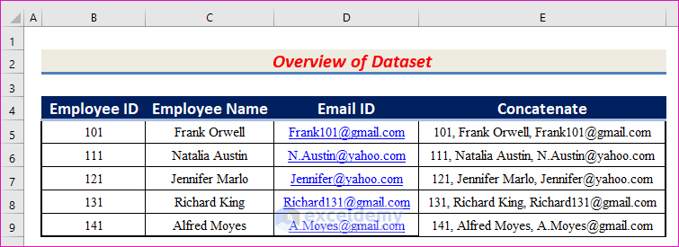
Consider the following dataset. We will use it to concatenate specific cells, merge a range of cells using the TEXTJOIN function, and nest the TEXTJOIN and FILTER functions as well in Excel.
Example 1 – Concatenate Specific Cells Using TEXTJOIN Function in Excel
Here we have a data set with the IDs, Names, and Email IDs of some employees of a company named Marco Group. We can use the TEXTJOIN function to merge all information about each employee into a single text value separated by commas(,).
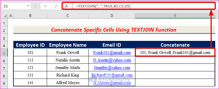
- Copy the following formula in cell E5 for the first employee:
=TEXTJOIN(", ",TRUE,B5,C5,D5)“, “ is the delimiter, TRUE is the ignore_empty, B5, C5, and D5 is the text 1, text2, and text 3 respectively of the TEXTJOIN function.
- Press Enter on your keyboard. The return is 101, Frank Orwell, [email protected].
- AutoFill the TEXTJOIN function to the rest of the cells in the column.
- We have merged all information of each into single cells using the TEXTJOIN function.
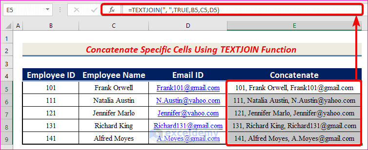
- We have used numbers (Employee ID) as well as strings (Name and Email ID) inside the TEXTJOIN function.
- The TEXTJOIN function can join both numbers and strings.
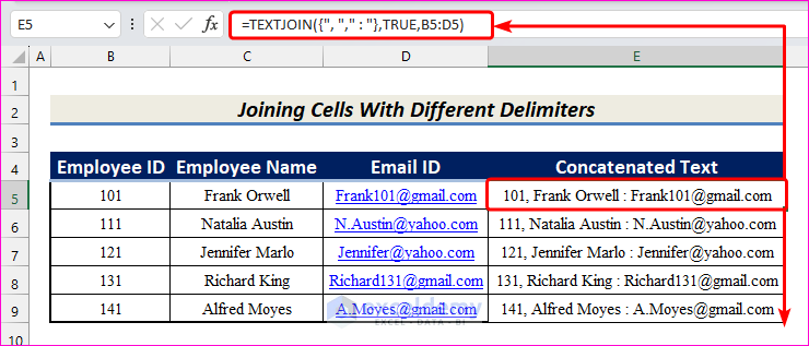
Example 2 – Joining Cells With Different Delimiters
- Apply the following formula in cell E5 to join cells with different delimiters, press Enter, and drag the Fill Handle up to cell E9:
=TEXTJOIN({", "," : "},TRUE,B5:D5)Here, {“, “,” : “} are the set of delimiters we will use, and B5:D5 is the range of cells to join.
As a result, you will have the selected cells joined by two delimiters as shown in the image below.
Example 3 – Merge a Range of Values by Applying TEXTJOIN Function in Excel
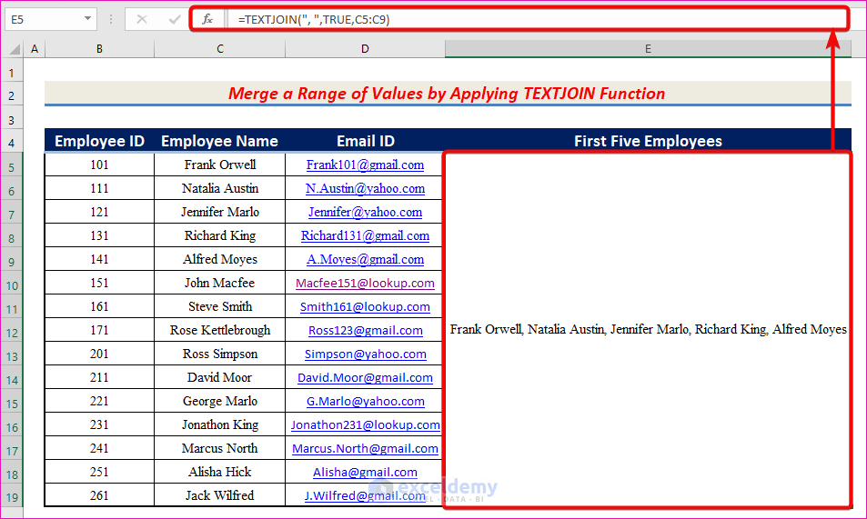
In the above data set, you can use the TEXTJOIN function to merge the names of the first five employees using this formula.
- Insert this formula in cell E5:
=TEXTJOIN(", ",TRUE,C5:C9)- Press Enter on your keyboard to get the result. The output for the sample is Frank Orwell, Natalia Austin, Jennifer Marlo, Richard King, and Alfred Moyes.
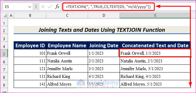
Example 4 – Joining Texts and Dates Using TEXTJOIN Function
- Use the formula given below in cell E5 to join the texts and dates together:
=TEXTJOIN(", ",TRUE,C5,TEXT(D5, "m/d/yyyy"))- Press Enter and use AutoFill through the column.
- The texts and dates will be concatenated as demonstrated in the following image.
Formula Breakdown
- TEXT(D5, “m/d/yyyy”) → Here, the TEXT function is used to convert the numerical date value to date format.
- D5 → It is the value argument.
- “m/d/yyyy” → This refers to the format_text argument.
- Output → “1/1/2023”.
- TEXTJOIN(“, “,TRUE,C5,TEXT(D5, “m/d/yyyy”)) → TEXTJOIN(“, “,TRUE,C5,”1/1/2023”)
- “, “ → It is the delimiter argument.
- TRUE → This represents the ignore_empty argument.
- C5 → It refers to the text1 argument.
- “1/1/2023” → This indicates the [text2] argument.
- Output → Frank Orwell, 1/1/2023.
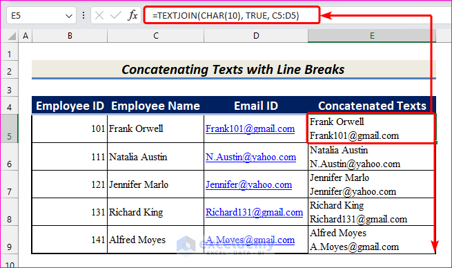
Example 5 – Concatenating Texts with Line Breaks
- Use the following formula in cell E5, press Enter, and drag the Fill Handle to copy the formula for the remaining cells:
=TEXTJOIN(CHAR(10), TRUE, C5:D5)Here, the CHAR function is used to give a line break (character with ASCII code 10) between two texts, and C5:D5 denotes the range of cells to concatenate.
Example 6 – Using TEXTJOIN Function with Criteria
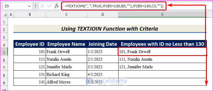
- Apply the formula below in cell E5:
=TEXTJOIN(", ",TRUE,IF(B5<130,B5,""),IF(B5<130,C5,""))- Hit Enter.
- Use the Fill Handle to copy the formula for the remaining cells.
- As a result, you have the concatenated Employee Name, and Employee ID where the Employee ID is less than 130.
Formula Breakdown
- IF(B5<130,B5,””) → The IF function checks whether the Employee ID is less than 130 or not.
- B5<130 → This is the logical_test argument.
- B5 → It refers to the [value_if_true] argument.
- “” → This indicates the [value_if_false] argument.
- Output → 101.
- IF(B5<130,C5,””) → This IF function also checks for the same condition as the previous one.
- Output → “Frank Orwell”.
- TEXTJOIN(“, “,TRUE,IF(B5<130,B5,””),IF(B5<130,C5,””)) → TEXTJOIN(“, “,TRUE,101,”Frank Orwell”)
- Output → 101, Frank Orwell.
Example 7 – Combine Texts with Multiple Criteria by Nesting TEXTJOIN and FILTER Functions
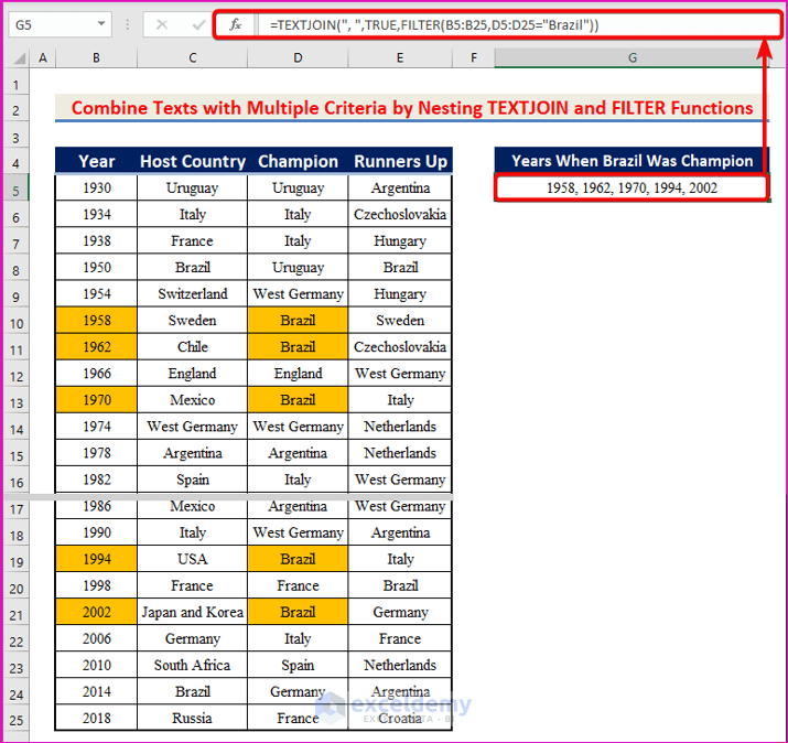
Here we have a new data set with the Years, Host Countries, Champions, and Runners-ups of the FIFA World Cup from 1930 to 2018. Let’s display the years in which Brazil became the champion in a single cell.
- Copy the following formula in cell G5 to merge the years in a single cell, separated by commas(,):
=TEXTJOIN(", ",TRUE,FILTER(B5:B25,D5:D25="Brazil"))- You can use the TEXTJOIN function with any array formula to merge the results into a single cell.
Formula Breakdown
- FILTER(B5:B25,D5:D25=”Brazil”) will return an array of the years in which Brazil became the champion.
- After that, TEXTJOIN(“, “,TRUE,FILTER(B5:B25,D5:D25=”Brazil”)) will concatenate the years in which Brazil became the champion in one cell.
Reasons Behind TEXTJOIN Function Not Working in Excel
| Errors | When They Show |
|---|---|
| #VALUE! | Shows when any argument in the function is missing, or any argument is of the wrong data type. |
| #NAME! | While using the older version (before Excel 2019) which is not capable of the TEXTJOIN function. |
| #NULL! | This happens when we fail to separate the strings that we want to join with a comma. |
Things to Remember
- Using the TEXTJOIN function, you can join up to 252 text arguments.
- TEXTJOIN function is available in Excel from Excel 2019. So, if you are using an older version of Excel then you need to use alternatives to the TEXTJOIN function like the CONCATENATE function.
Frequently Asked Questions
1. What is the difference between the CONACTENATE function and the TEXTJOIN function?
The TEXJOIN function allows you to define any delimiter you want which can’t be done by the CONCATENATE function. Additionally, it is possible to ignore any empty cell from the resulting string while using the TEXTJOIN function. But the CONCATENATE function can’t do that.
2. What are some alternatives to the TEXTJOIN function?
As an alternative, you can concatenate text using the CONCATENATE function. You can also use the & operator to join texts. But, these alternatives are not as efficient as the TEXTJOIN function.
Download Practice Workbook
Download this practice workbook to follow along while you are reading this article.
<< Go Back to Excel Functions | Learn Excel
Get FREE Advanced Excel Exercises with Solutions!


I have a column of dates and several columns of subjects (they’re being fed by a form). To look something like this:
Date | SubjectA | SubjectB |…etc
I want to create a text cell (right now I have it in the footer of each subjects column) that concatenates date with text notes for each subject:
So the contents of the footer cell can look something like this:
Jan 6, 2024 random note for Subject A yaddah yaddah (entered on 1/6/24)
Feb 4 2024 another random note for Subject A Ipsum Loorum (entered on 2/4/24)
Any thoughts?
Hello Kevin O’Boyle,
To achieve this, you can use the TEXTJOIN function to concatenate notes with the dates for each subject. Here’s an approach you might try:
1. In the footer cell for each subject, use TEXTJOIN with the delimiter you want (like a line break).
2. Format your entries using a combination of TEXT (for the date) and CONCATENATE (for text and notes).
Example formula for the footer cell:
=TEXTJOIN(CHAR(10), TRUE, IF(A2:A10<>“”, TEXT(A2:A10, “mmm d, yyyy”) & ” ” & B2:B10 & ” (entered on ” & TEXT(A2:A10, “m/d/yy”) & “)”, “”))
Replace A2:A10 with your date range and B2:B10 with notes. This will list each entry on a new line with the formatted date and note text.
Regards
ExcelDemy