How to Create Training Attendance Sheet in Excel

In our daily corporate life or in the case of any organization, we need to count the attendance of the employees. If you are curious to learn how you can create training attendance sheets in Excel, then this article may come in handy for you. In this article, we discuss how you can create a training attendance sheet in Excel with elaborate explanations.

How to Create Training Attendance Sheet in Excel: with Easy Steps

A training attendance sheet normally resembles a typical attendance sheet, You need to summarise trainee information and their time spent in the training.

For avoiding any version or compatibility issues, try to use the Microsoft 365 version.

Step 1: Prepare Outline

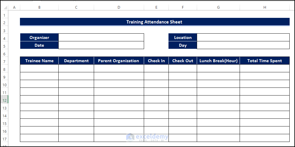
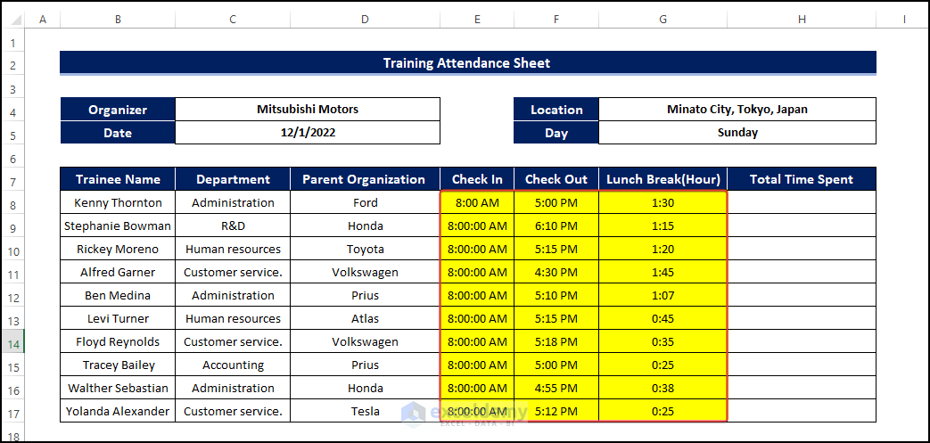
Before we delve into creating the Attendance sheet, we need to prepare the outline first.

To create a trainee attendance, we need to create a template or structure for the attendance.
For this, we created the below structure mentioned below.
We got the Organizer, Date, Location, and Day of the training.
And in the below table, you need to Trainee Name, Department, Parent Organization(from where they come to attend the training), Check-In time, Check-Out time, Lunch Break, and finally, the Total Time Spent.

Step 2: Assign Date and Day

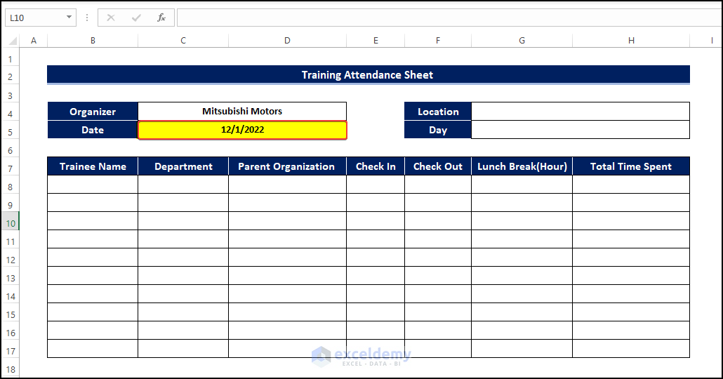
In the next stage, we can start putting the values in the sheets. We put the organizer’s name and the date in the template. To extract the Day name from the date, we are going to use the DAY function.

Enter the date of the training and the organizer’s name.

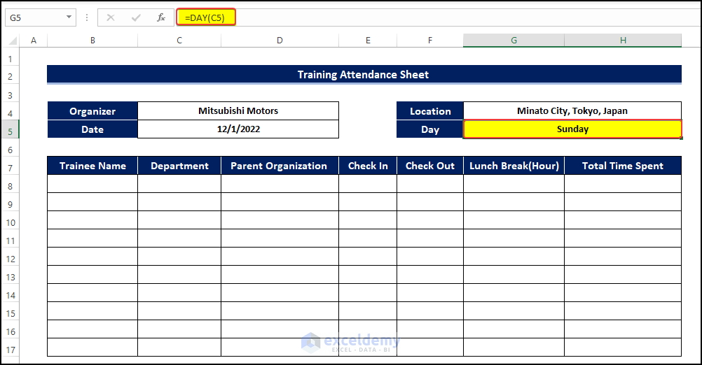
We also want to know the day of the training date, to do this, select the cell G5 and enter the following formula:

=DAY(C5)

After entering the formula, we got the day of the date mentioned in cell C5.

Step 3: Allocate Check In, Check Out, Lunch Break and Parent Organization Name

Now we have the preliminary data of training, we can now add the most important feature of the attendance sheets. They are the names and the time of their checking in or out.

Now we can enter the trainee’s name and the department name to which they will be assigned.
Moreover, enter the Parent Organization name from which they are coming to the Parent Organization column.

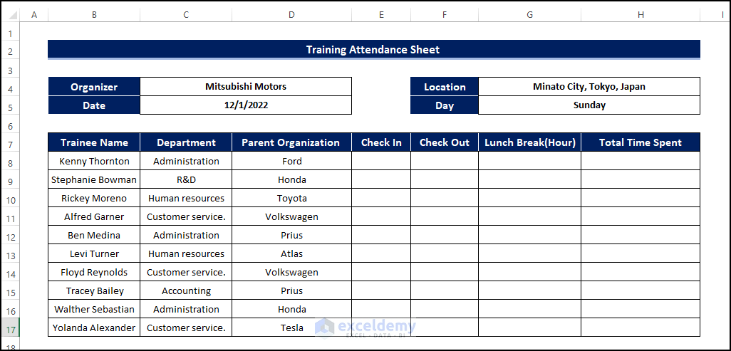
After filling up the column, we can see that the people are coming from diverse organizations.
Now it’s time to put the time of trainees checking in and checking out in the sheet.

Step 4: Calculate Total Time

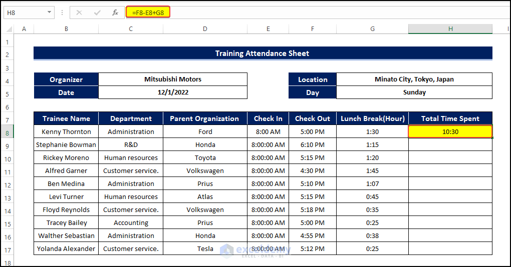
Now we have all the necessary information, we can calculate the total time spent of each employee.

Select the cell H8 and enter the following formula:

=F8-E8+G8

Entering this formula will calculate the total time spent each day minus the Lunch Time.

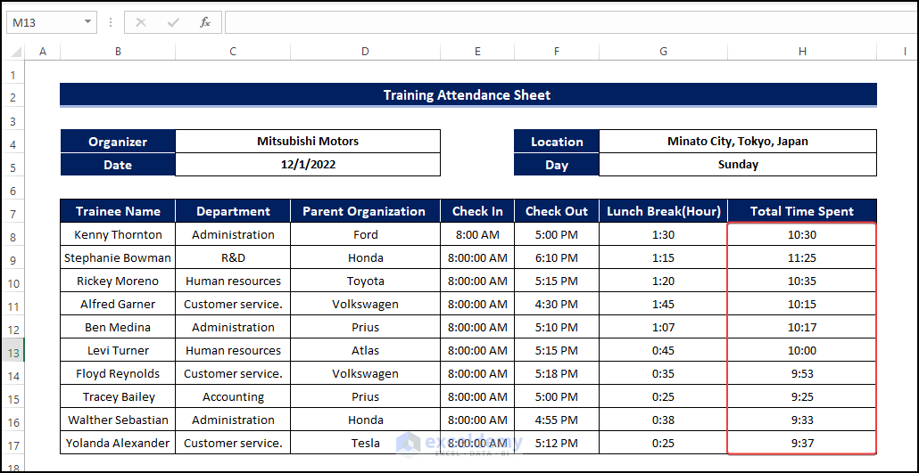
Then drag the Fill Handle to cell H17.
Doing this will calculate the total time spent on each employee.

How to Make a Class Attendance Sheet in Excel

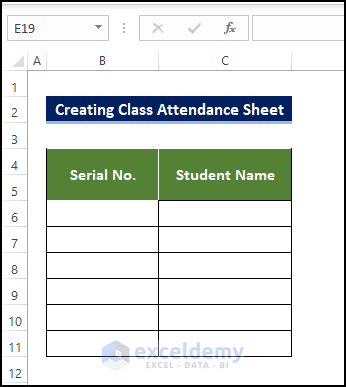
In the following section, we will create a simple and ready-to-use monthly class attendance sheet with predefined formulas to save a huge amount of time.

Step 1: Add Serial No. and Student Name Column

In this first step, we will add 2 columns to denote the student’s serial number and name. We will also insert some sample names inside our datasheet.

First, click on cell B5 and type Serial No.
Next, select cell C5 and type Student Name.
Here, you will enter the students’ names and serial numbers.

Step 2: Type Month Name and Days

We will be making this attendance sheet using January as the sample month. So, we will insert 31 columns representing each day of the month.

To begin this step, enter the month name in cell D4 and merge cells from D4 to AH4.
Next, enter the days starting from cell D5.
Note that, after filling the first few days, you can drag the Fill Handle to the right to fill the series.
Not only this, we will mark the weekends with specially formatted cells.

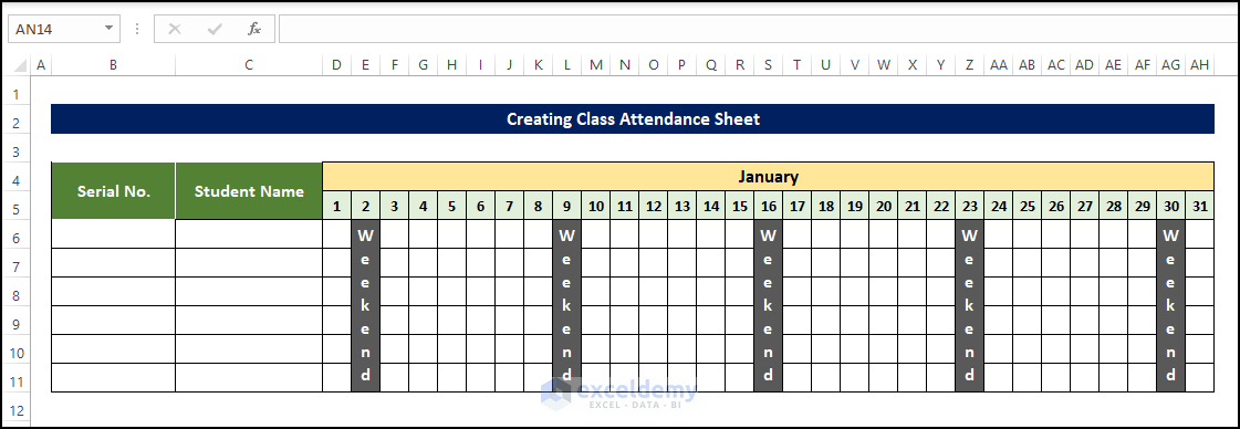
Step 3: Insert Absent and Present Columns

In this step, we will add two more columns to count the days a student was absent or present. This is a premade function in excel that counts the number of cells in a range that fulfills a specified condition.

Next, click on cell AI and enter the Absent column header.
Similarly, go to cell AJ and type the column header Present.

Step 4: Formulate Absence and Present Column

Now that our attendance sheet is complete, we will try it out by inserting attendance data for each student. Here we will use P to indicate a student is present and A to indicate absent.For this, we will apply the COUNTIF function.

Here, enter student attendance data in the empty cells for each day.
Also, as you enter the Present or Absent student data, the formula of column AI and AJ will start counting them.

Now, select cell AI6 and enter the following formula:

=COUNTIF(D6:AH6,”A”)

Then drag the Fill Handle to cell AI11.

Now select cell AJ6 and enter the following formula:

=COUNTIF(D6:AH6,”P”)

Then drag the Fill Handle to cell AJ11.

Doing this will fill the range of cell AJ6:AJ11 with the number of present days of each student.

💬 Things to Remember

You may want to add some conditional formatting to the data to make it more visual. But try not to make this too complex.
Try to understand the core structure of the sheet and how to enter data inside it.
If there occur any changes to your student’s data, make sure to modify them accordingly before entering the data for a new month.
Remember that, you only need to enter the student’s information once and then copy them to the sheets for other months.
If you have a large number of students, you can expand this sheet to fit your needs.

Download Practice Workbook

Download this practice workbook below.

Training Attendance Sheet.xlsx

Conclusion

To sum it up, the issue of how we can create a training attendance sheet in Excel using 4 separate steps.

For this problem, a workbook is available to download where you can practice these methods.

Feel free to ask any questions or feedback through the comment section.

<< Go Back to Employee Attendance Sheet Excel | Excel HR Templates | Excel Templates

Get FREE Advanced Excel Exercises with Solutions!