Download the Workbook
4 Ways to Transpose Duplicate Rows to Columns in Excel
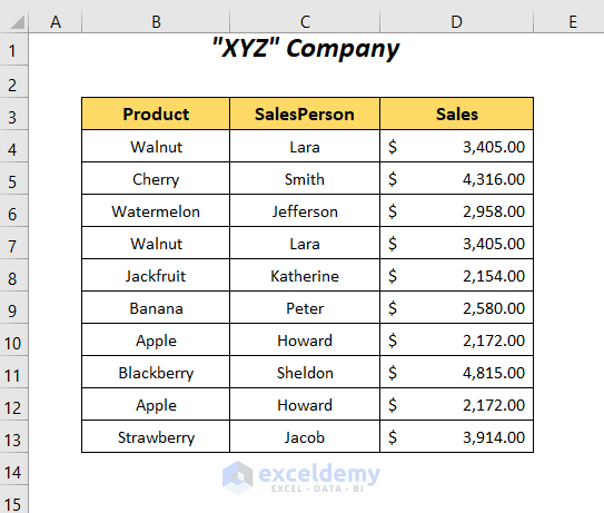
We have the following dataset containing the sales records of different products, with some repeat rows. We will convert the duplicate rows into columns.
Method 1 – Using Conditional Formatting to Transpose Duplicate Rows to Columns
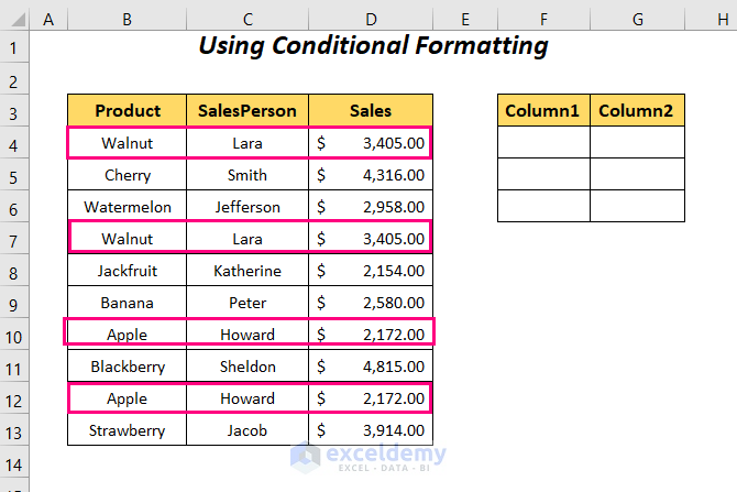
We will use Conditional Formatting to highlight the duplicate rows then transpose them in the Column1 and Column2 columns.
Steps:
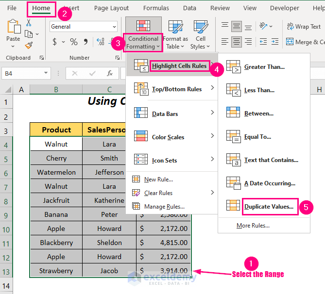
- Select the data range and then go to the Home tab,
- Choose Conditional Formatting, go to the Highlight Cells Rules option, and select the Duplicate Values option.
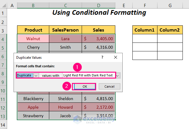
The Duplicate Values dialog box will appear.
- Choose Duplicate and Light Red Fill with Dark Red Text options in the Format cells that contain box.
- Press OK.
The duplicate rows for the products Walnut and Apple will be highlighted.
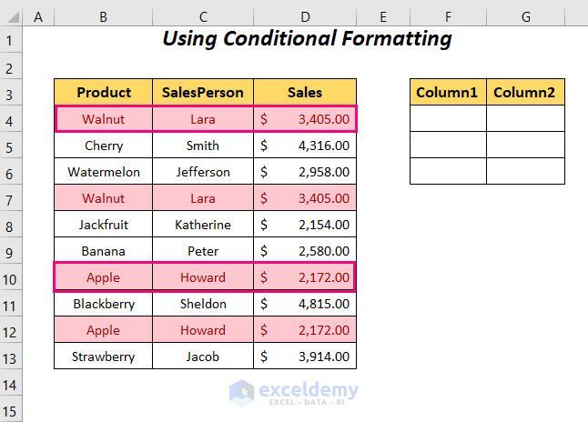
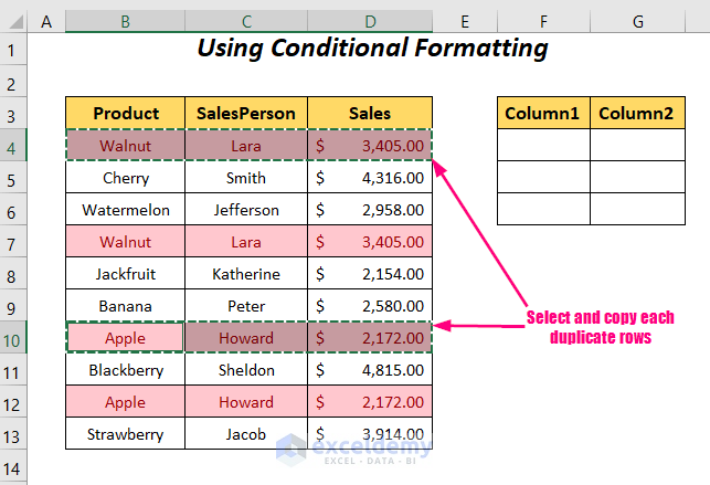
- Select the rows for the products Walnut and Apple by holding Ctrl while selecting.
- Press Ctrl + C.
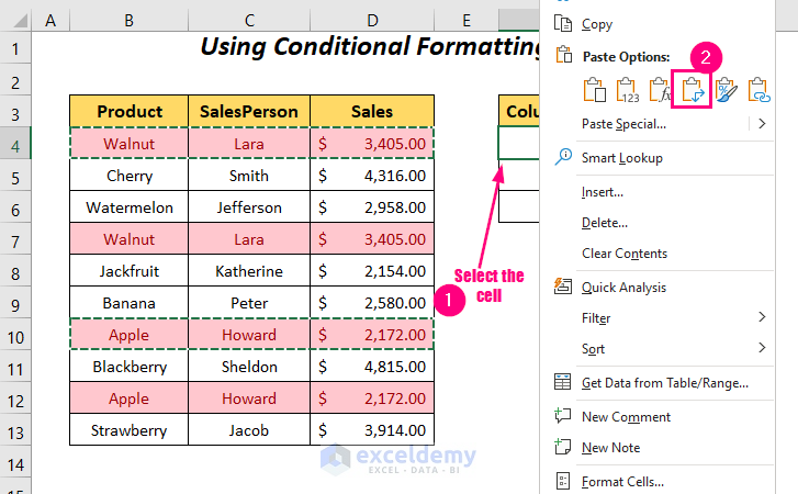
- Right-click on the destination cell and select the Paste Transposed option.
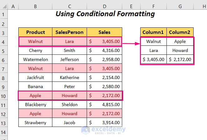
This will transpose the duplicate rows to columns.
Read More: Conditional Transpose in Excel (2 Examples)
Method 2 – Using the COUNTIF Function
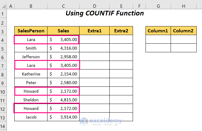
We will combine the names of the salespersons and sales values with the Ampersand operator in the Extra1 column, then count the number of repetitions of the rows with the COUNTIF function in the Extra2 column. We will convert the repeated rows to columns using the Transpose option.
Steps:
- Insert the following formula in cell D4 to combine all of the cells of each row.
=B4&C4B4 is the name of the SalesPerson, C4 is the Sales value, and & will join them.
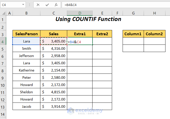
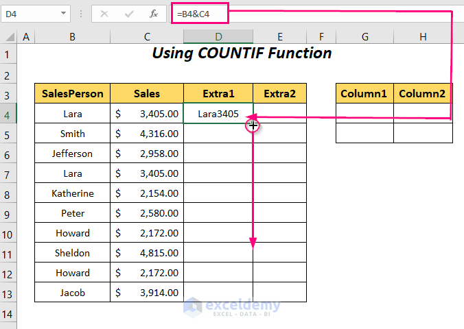
- Press Enter and drag down the Fill Handle tool.
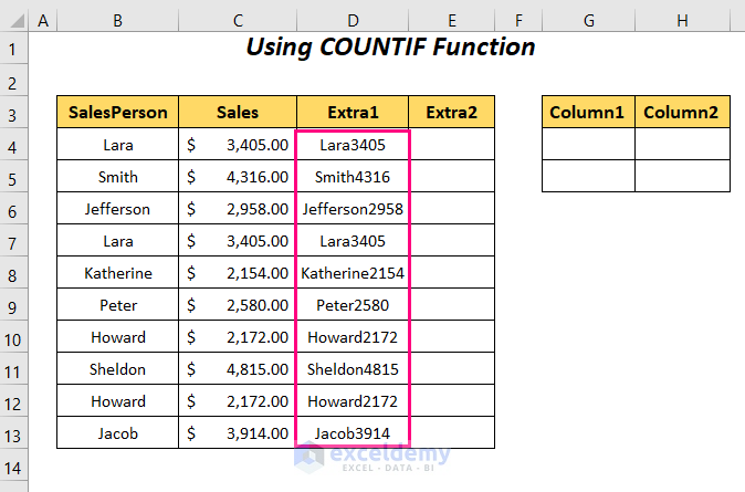
You will get the combination of the cells of each row in the Extra1 column.
- To count the repetitions of the rows of the Extra1 column, use the following formula in cell E4.
=COUNTIF($D$4:D4,D4)D4 is the criteria and $D$4:D4 is the range and this range will be from the starting row to the row up to which the formula is used, such as for Row 8 the range will be $D$4:D8.
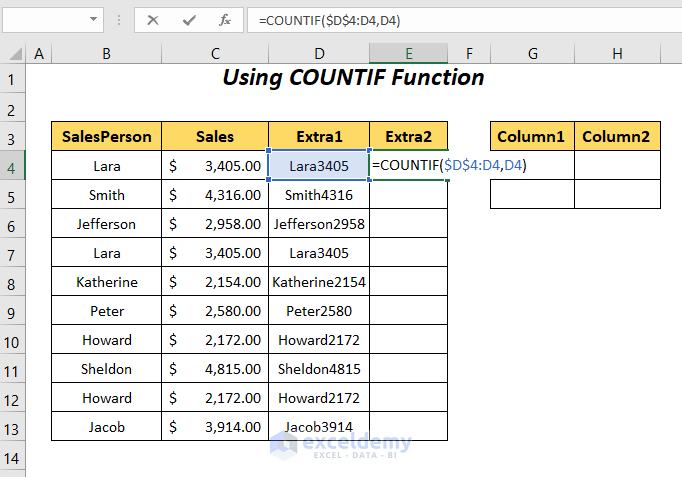
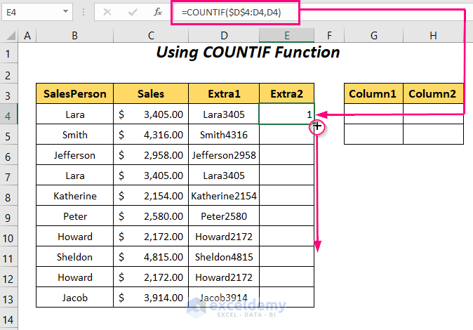
- Press Enter and drag down the Fill Handle tool.
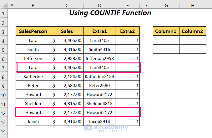
You will get the number of repetitions in the Extra2 column. Here, 2 for Lara and Howard means they appeared twice with their sales values. We will convert those rows.
- Select the rows for Lara and Howard by holding Ctrl while selecting them, then press Ctrl + C.
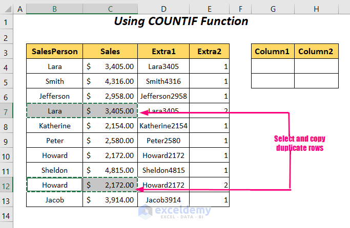
- Right-click on the destination cell and select the Transpose option from Paste Options.
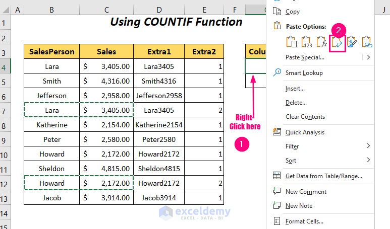
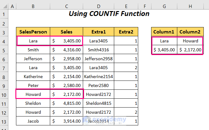
This transposes the duplicate rows for Lara and Howard as columns.
Read More: How to Transpose Rows to Columns in Excel (5 Useful Methods)
Similar Readings
- How to Transpose Every n Rows to Columns in Excel (2 Easy Methods)
- Excel Power Query: Transpose Rows to Columns (Step-by-Step Guide)
- Transpose Multiple Columns into One Column in Excel (3 Handy Methods)
Method 3 – Using a Combination of IF and COUNTIFS Functions
We are going to use the IF and COUNTIFS functions to detect whether the row is duplicate.
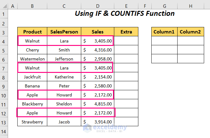
Steps:
- Use the following formula in cell E4.
=IF(COUNTIFS($B$4:$B$13,$B4,$C$4:$C$13,$C4,$D$4:$D$13,$D4)>1, "Repeated Row", "")$B$4:$B$13, $C$4:$C$13, and $D$4:$D$13 are the first, second, and third ranges. $B4, $C4, and $D4 are the first, second, and third criteria.
- COUNTIFS($B$4:$B$13,$B4,$C$4:$C$13,$C4,$D$4:$D$13,$D4) → returns a number that represents the number of repetitions of the rows.
Output → 2
- COUNTIFS($B$4:$B$13,$B4,$C$4:$C$13,$C4,$D$4:$D$13,$D4)>1 becomes
2>1 → returns TRUE for fulfilling the condition otherwise FALSE.
Output → TRUE
- IF(COUNTIFS($B$4:$B$13,$B4,$C$4:$C$13,$C4,$D$4:$D$13,$D4)>1, “Repeated Row”, “”) becomes
IF(TRUE, “Repeated Row”, “”) → returns the string “Repeated Row” for TRUE, otherwise a blank.
Output → Repeated Row
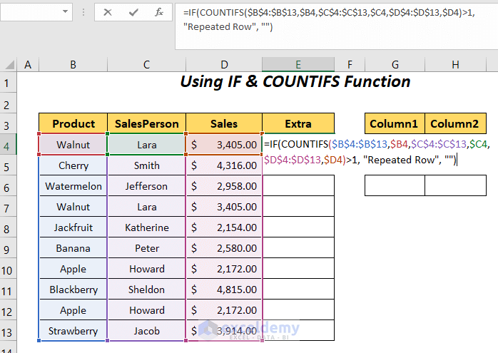
- Press Enter and drag down the Fill Handle tool.
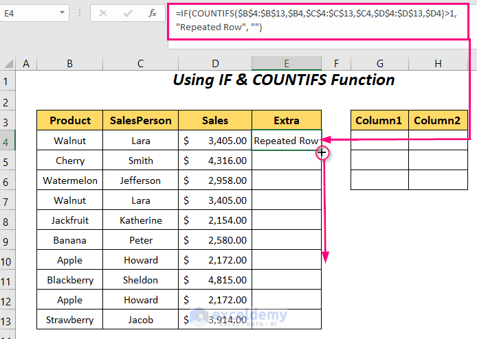
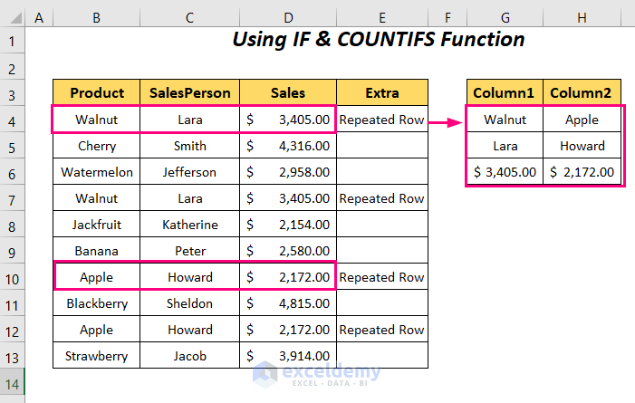
We are getting the text string Repeated Row for the duplicate rows.
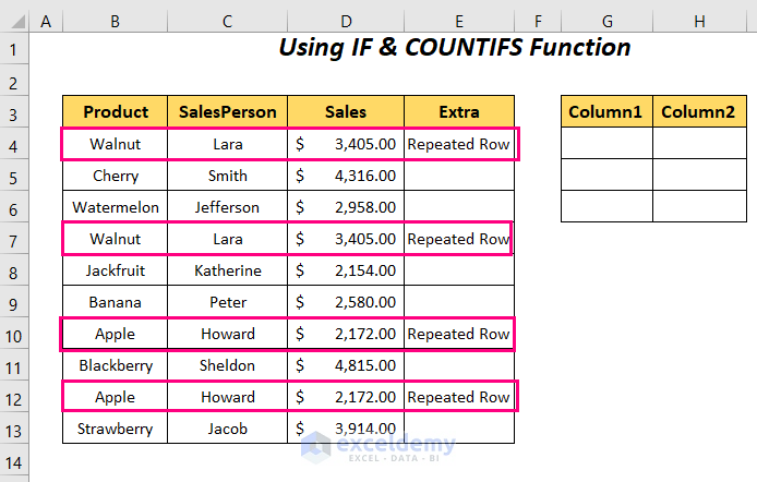
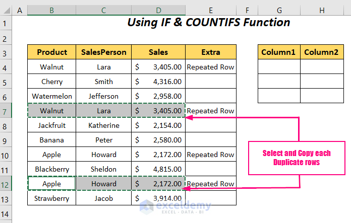
- Select the rows for the products Walnut and Apple by holding Ctrl while selecting them, then press Ctrl + C.
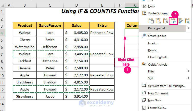
- Right-click on the destination cell and select the Transpose option from Paste Options.
We are getting the transposed duplicate rows like the following figure.
Read More: How to Transpose Rows to Columns Based on Criteria in Excel (2 Ways)
Method 4 – Using VBA Code to Transpose Duplicate Rows to Columns in Excel
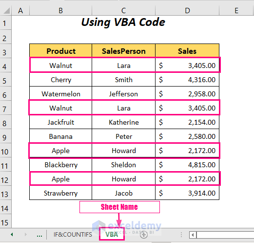
We’ll use the same dataset as before.
Steps:
- Go to the Developer tab and select the Visual Basic option.
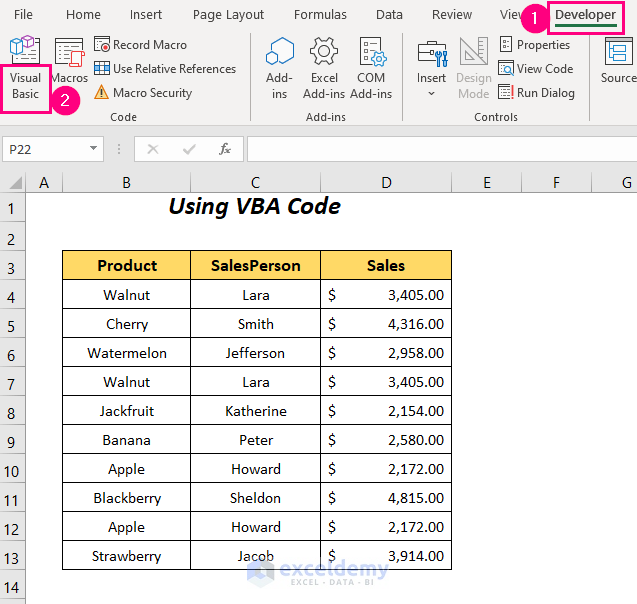
The Visual Basic Editor will open up.
- Go to the Insert tab and select Module.
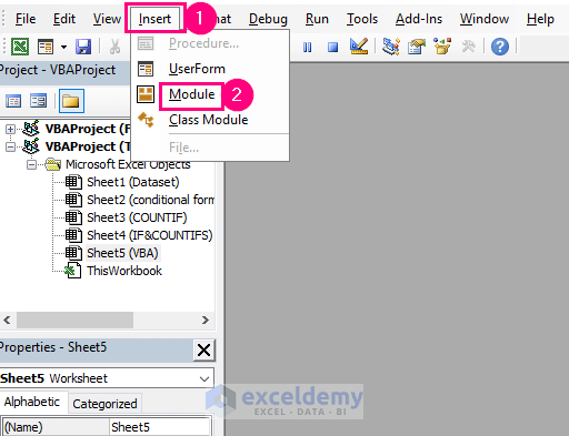
A Module will be created.
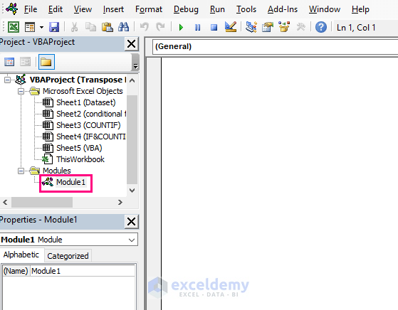
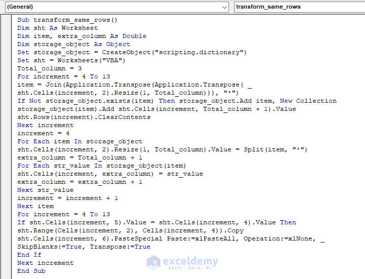
- Insert the following code in the module:
Sub transform_same_rows()
Dim sht As Worksheet
Dim item, extra_column As Double
Dim storage_object As Object
Set storage_object = CreateObject("scripting.dictionary")
Set sht = Worksheets("VBA")
Total_column = 3
For increment = 4 To 13
item = Join(Application.Transpose(Application.Transpose( _
sht.Cells(increment, 2).Resize(1, Total_column))), "*")
If Not storage_object.exists(item) Then storage_object.Add item, New Collection
storage_object(item).Add sht.Cells(increment, Total_column + 1).Value
sht.Rows(increment).ClearContents
Next increment
increment = 4
For Each item In storage_object
sht.Cells(increment, 2).Resize(1, Total_column).Value = Split(item, "*")
extra_column = Total_column + 1
For Each str_value In storage_object(item)
sht.Cells(increment, extra_column) = str_value
extra_column = extra_column + 1
Next str_value
increment = increment + 1
Next item
For increment = 4 To 13
If sht.Cells(increment, 5).Value = sht.Cells(increment, 4).Value Then
sht.Range(Cells(increment, 2), Cells(increment, 4)).Copy
sht.Cells(increment, 6).PasteSpecial Paste:=xlPasteAll, Operation:=xlNone, _
SkipBlanks:=True, Transpose:=True
End If
Next increment
End Sub
We have declared sht as Worksheet, item, extra_column as Double, storage_object as Object, and then set sht to the worksheet VBA and assigned Total_column to 3.
storage_object is set to the Dictionary object which will help us to store items here.
We have used the FOR loop for a range of increments from row 4 to 13, and then using the TRANSPOSE function twice and then the JOIN function we have combined all of the cells of the rows with a separator * to the variable item. After that, we added the items to the storage_object and then we cleared all of the rows.
The unique rows will be entered into the three columns by using the SPLIT function and then the sales values for the duplicate rows will be added to the adjacent column of the Sales column.
Using the IF statement, we will check the sales values to the values of the adjacent cells. If the condition is fulfilled, we will copy that corresponding row and transpose it.
- Press F5.
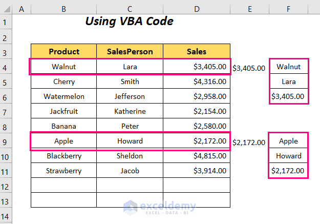
Read More: How to Transpose Rows to Columns Using Excel VBA (4 Ideal Examples)
Practice Section
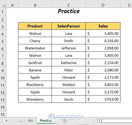
We have provided a Practice section like below in a sheet named Practice.
Further Readings
- How to Transpose in Excel (5 Easy Ways)
- Transpose Multiple Rows in Group to Columns in Excel
- How to Transpose Columns to Rows In Excel (6 Methods)
- Convert Columns to Rows in Excel Using Power Query
- How to Convert Columns to Rows in Excel Based On Cell Value
- VBA to Transpose Multiple Columns into Rows in Excel (2 Methods)
- How to Convert Column to Comma Separated List With Single Quotes
- How to Transpose in Excel VBA (3 Methods)


